Snow Modeling
Contents
Snow Modeling
Contributors: Melissa Wrzesien1,2, Brendan McAndrew1,3, Jian Li4,5, Caleb Spradlin4,6
1 Hydrological Sciences Lab, NASA Goddard Space Flight Center, 2 University of Maryland, 3 Science Systems and Applications, Inc., 4 InuTeq, LLC, 5 Computational and Information Sciences and Technology Office (CISTO), NASA Goddard Space Flight Center, 6 High Performance Computing, NASA Goddard Space Flight Center
Learning Objectives
Learn about the role of modeling in a satellite mission
Open, explore, and visualize gridded model output
Compare model output to raster- and point-based observation datasets
The goal of a future snow satellite is to provide improved understanding of global snow mass, as compared to current estimates. However, a single sensor likely won’t be able to accurately observe all types of snow in all conditions for the entire globe. Instead, we need to combine future snow observations with other tools - including models and observations from currently available satellites.
Models can also help to extend snow observations to areas where observations are not available. Data may be missing due to orbit gaps or masked out in regions of higher uncertainty. Remote sensing observations and models can be combined through data assimilation, a process where observations are used to constrain model estimates.
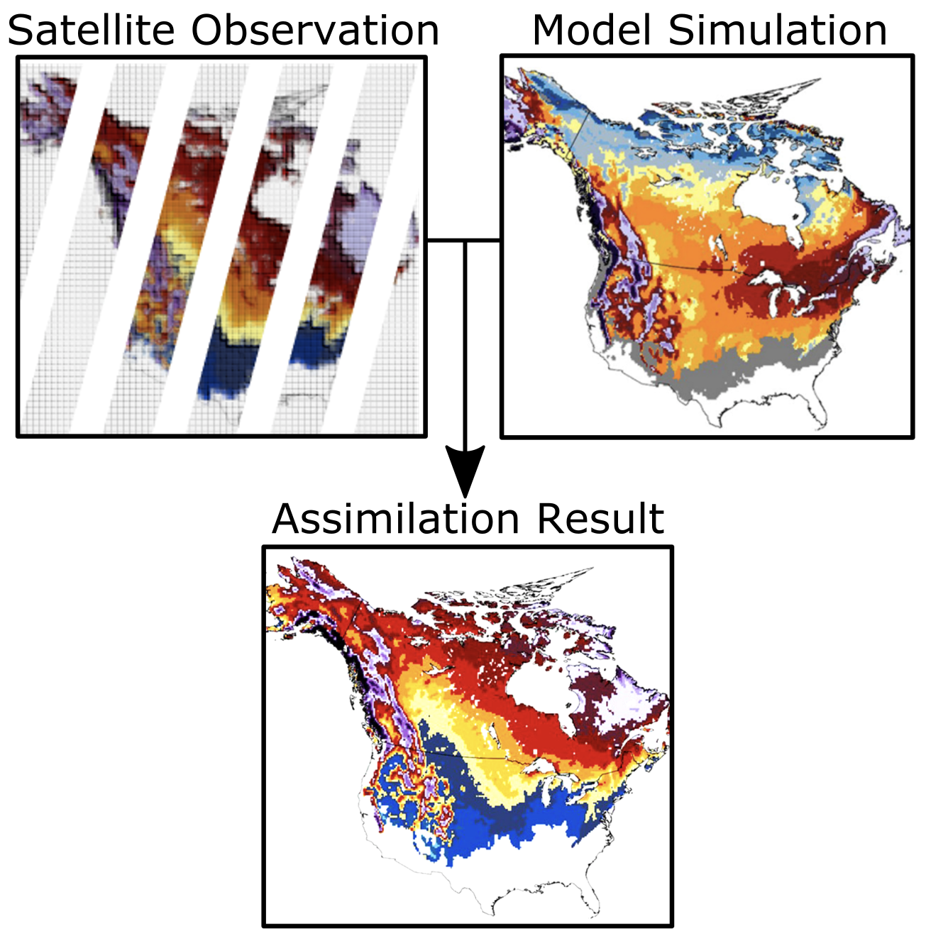
The figure above shows a conceptual example of how satellite observations with orbit gaps could be combined with a model to produce results with no missing data. (Figure modified from diagram provided by Eunsang Cho)
What is LIS?
Since models will likely play a role in processing observations from a snow satellite mission, it is important to become comfortable working with gridded data products. Today we will use sample model output from NASA’s Land Information System (LIS).
The Land Information System is a software framework for land surface modeling and data assimilation developed with the goal of integrating satellite and ground-based observational data products with advanced modeling techniques to produce estimates of land surface states and fluxes.
TL;DR LIS = land surface models + data assimilation
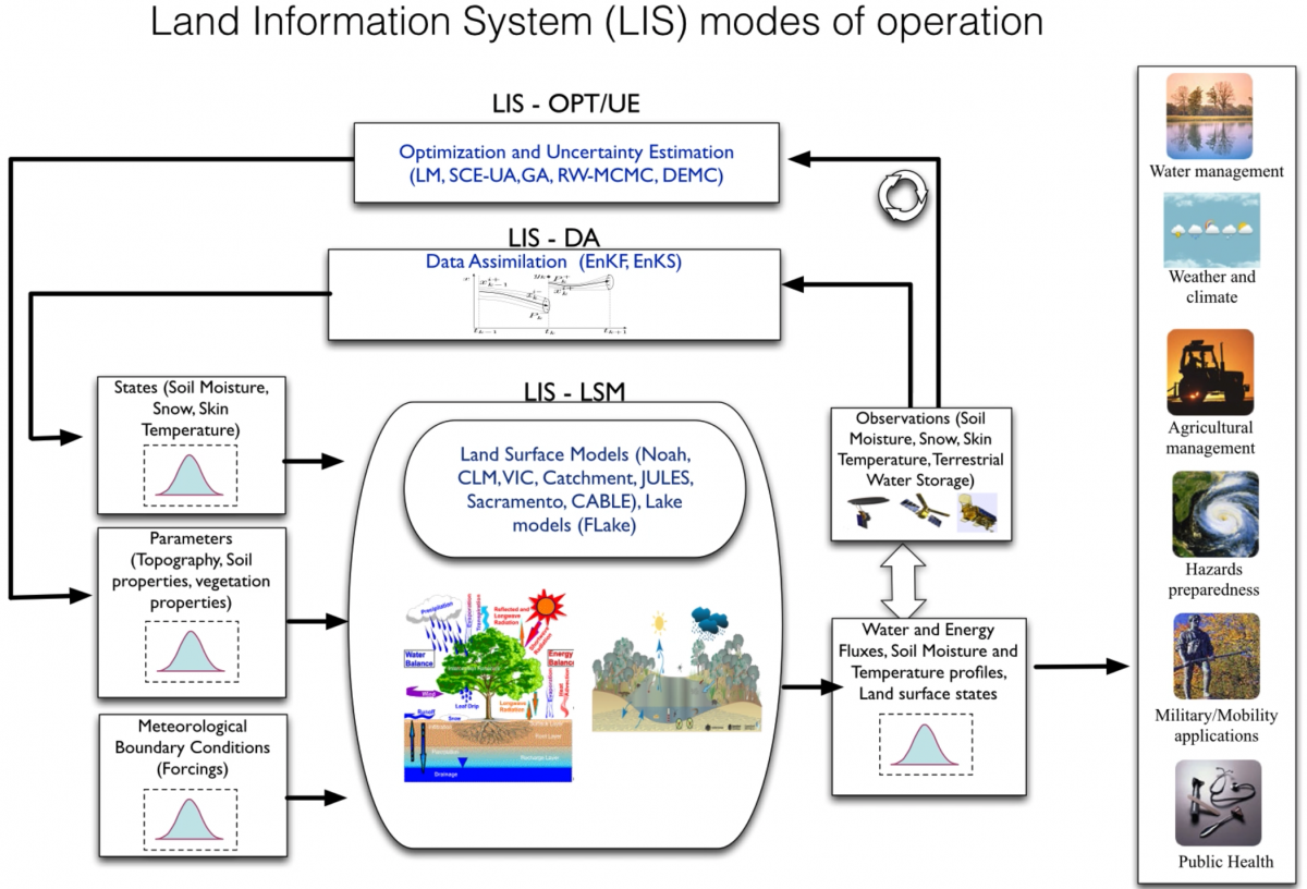
One key feature LIS provides is flexibility to meet user needs. LIS consists of a collection of plug-ins, or modules, that allow users to design simulations with their choice of land surface model, meteorological forcing, data assimilation, hydrological routing, land surface parameters, and more. The plug-in based design also provides extensibility, making it easier to add new functionality to the LIS framework.
Current efforts to expand support for snow modeling include implementation of snow modules, such as SnowModel and Crocus, into the LIS framework. These models, when run at the scale of ~100 meters, will enable simulation of wind redistribution, snow grain size, and other important processes for more accurate snow modeling.
Development of LIS is led by the Hydrological Sciences Laboratory at NASA’s Goddard Space Flight Center. (Figure above provided by the LIS team)
Working with Modeled Output
Here we will use sample model output from a LIS-SnowModel simulation over a western Colorado domain. Daily estimates of SWE, snow depth, and snow density are written to output. The SnowModel simulation has a spatial resolution of 100 m. We’ve provided four years of output, though here we’ll mostly use output from water year 2020.
Below, we’ll walk through how to open and interact with the LIS-SnowModel output. Our main objectives are to demonstrate how to do the following with a gridded dataset like LIS-SnowModel:
Understand attributes of model data file and available variables
Create a spatial map of model output
Create time series at a point and averaged across domain
Compare LIS-SnowModel to raster and point data
Create a visualization for quick evaluation of model estimates
Import Libraries
# interface to Amazon S3 filesystem
import s3fs
# interact with n-d arrays
import numpy as np
import xarray as xr
# interact with tabular data (incl. spatial)
import pandas as pd
import geopandas as gpd
# interactive plots
import holoviews as hv
import geoviews as gv
import hvplot.pandas
import hvplot.xarray
# set bokeh as the holoviews plotting backend
#hv.extension('bokeh')
# set holoviews backend to Bokeh
#gv.extension('bokeh')
# used to find nearest grid cell to a given location
from scipy.spatial import distance
import fsspec
from datetime import datetime as dt
from geoviews import opts
from geoviews import tile_sources as gvts
from datashader.colors import viridis
import datashader
from holoviews.operation.datashader import datashade, shade, dynspread, spread, rasterize
from holoviews.streams import Selection1D, Params
import panel as pn
import param as pm
import warnings
import holoviews.operation.datashader as hd
warnings.filterwarnings("ignore")
pn.extension()
pn.param.ParamMethod.loading_indicator =True
Load the LIS-SnowModel Output
The xarray library makes working with labelled n-dimensional arrays easy and efficient. If you’re familiar with the pandas library it should feel pretty familiar.
Here we load the LIS-SnowModel output into an xarray.Dataset object:
# create S3 filesystem object
s3 = s3fs.S3FileSystem(anon=False)
# define the name of our S3 bucket
bucket_name = 'eis-dh-hydro/SNOWEX-HACKWEEK'
# define path to store on S3
lis_output_s3_path_time_chunk = f's3://{bucket_name}/2022/ZARR/SURFACEMODEL/LIS_HIST_rechunkedV4.d01.zarr'
lis_output_s3_path = f's3://{bucket_name}/2022/ZARR/SURFACEMODEL/LIS_HIST_default_chunks.d01.zarr/'
# create key-value mapper for S3 object (required to read data stored on S3)
lis_output_mapper = s3.get_mapper(lis_output_s3_path)
lis_output_mapper_tc = s3.get_mapper(lis_output_s3_path_time_chunk)
# open the dataset
lis_output_ds = xr.open_zarr(lis_output_mapper, consolidated=True)
lis_output_ds_tc = xr.open_zarr(lis_output_mapper_tc, consolidated=True)
Explore the Data
Display an interactive widget for inspecting the dataset by running a cell containing the variable name. Expand the dropdown menus and click on the document and database icons to inspect the variables and attributes.
lis_output_ds
<xarray.Dataset>
Dimensions: (time: 1694, north_south: 6650, east_west: 4800)
Coordinates:
lat (time, north_south, east_west) float32 dask.array<chunksize=(1, 6650, 4800), meta=np.ndarray>
lon (time, north_south, east_west) float32 dask.array<chunksize=(1, 6650, 4800), meta=np.ndarray>
* time (time) datetime64[ns] 2016-09-02 ... 2021-04-22
Dimensions without coordinates: north_south, east_west
Data variables:
SM_SWE_inst (time, north_south, east_west) float32 dask.array<chunksize=(1, 6650, 4800), meta=np.ndarray>
SM_SnowDensity_inst (time, north_south, east_west) float32 dask.array<chunksize=(1, 6650, 4800), meta=np.ndarray>
SM_SnowDepth_inst (time, north_south, east_west) float32 dask.array<chunksize=(1, 6650, 4800), meta=np.ndarray>
Attributes: (12/18)
DX: 0.10000000149011612
DY: 0.10000000149011612
MAP_PROJECTION: LAMBERT CONFORMAL
NUM_SOIL_LAYERS: 1
SOIL_LAYER_THICKNESSES: 1.0
SOUTH_WEST_CORNER_LAT: 35.49998092651367
... ...
history: created on date: 2022-05-16T17:12:56.387
institution: NASA GSFC
missing_value: -9999.0
references: Kumar_etal_EMS_2006, Peters-Lidard_etal_ISSE_2007
source:
title: LIS land surface model outputAccessing Attributes
Dataset attributes (metadata) are accessible via the attrs attribute:
lis_output_ds.attrs
{'DX': 0.10000000149011612,
'DY': 0.10000000149011612,
'MAP_PROJECTION': 'LAMBERT CONFORMAL',
'NUM_SOIL_LAYERS': 1,
'SOIL_LAYER_THICKNESSES': 1.0,
'SOUTH_WEST_CORNER_LAT': 35.49998092651367,
'SOUTH_WEST_CORNER_LON': -109.50030517578125,
'STANDARD_LON': -106.75,
'TRUELAT1': 37.0,
'TRUELAT2': 40.0,
'comment': 'website: http://lis.gsfc.nasa.gov/',
'conventions': 'CF-1.6',
'history': 'created on date: 2022-05-16T17:12:56.387',
'institution': 'NASA GSFC',
'missing_value': -9999.0,
'references': 'Kumar_etal_EMS_2006, Peters-Lidard_etal_ISSE_2007',
'source': '',
'title': 'LIS land surface model output'}
Accessing Variables
Variables can be accessed using either dot notation or square bracket notation. Here we will stick with square bracket notation:
# square bracket notation
lis_output_ds['SM_SnowDepth_inst']
<xarray.DataArray 'SM_SnowDepth_inst' (time: 1694, north_south: 6650,
east_west: 4800)>
dask.array<open_dataset-c6d82014a30be2b9e8bf97ca3ffac825SM_SnowDepth_inst, shape=(1694, 6650, 4800), dtype=float32, chunksize=(1, 6650, 4800), chunktype=numpy.ndarray>
Coordinates:
lat (time, north_south, east_west) float32 dask.array<chunksize=(1, 6650, 4800), meta=np.ndarray>
lon (time, north_south, east_west) float32 dask.array<chunksize=(1, 6650, 4800), meta=np.ndarray>
* time (time) datetime64[ns] 2016-09-02 2016-09-03 ... 2021-04-22
Dimensions without coordinates: north_south, east_west
Attributes:
long_name: snow depth
standard_name: snow_depth
units: m
vmax: 999999986991104.0
vmin: -999999986991104.0Watch out for large datasets!
Note that the 4-ish years of model output (1694 daily time steps for a domain of size 6650 x 4800) has a size of over 200 gb! As we’ll see below, this is just for an area over western Colorado. If we’re interested in modeling the western United States or CONUS or even global at high resolution, we need to be prepared to work with some large datasets.
Dimensions and Coordinate Variables
The dimensions and coordinate variable fields put the “labelled” in “labelled n-dimensional arrays”:
Dimensions: labels for each dimension in the dataset (e.g.,
time)Coordinates: labels for indexing along dimensions (e.g.,
'2020-01-01')
We can use these labels to select, slice, and aggregate the dataset.
Subsetting in Space or Time
xarray provides two methods for selecting or subsetting along coordinate variables:
index selection:
ds.isel(time=0)value selection
ds.sel(time='2020-01-01')
For example, we can use value selection to select based on the the coorindates of a given dimension:
lis_output_ds.sel(time='2020-01-01')
<xarray.Dataset>
Dimensions: (north_south: 6650, east_west: 4800)
Coordinates:
lat (north_south, east_west) float32 dask.array<chunksize=(6650, 4800), meta=np.ndarray>
lon (north_south, east_west) float32 dask.array<chunksize=(6650, 4800), meta=np.ndarray>
time datetime64[ns] 2020-01-01
Dimensions without coordinates: north_south, east_west
Data variables:
SM_SWE_inst (north_south, east_west) float32 dask.array<chunksize=(6650, 4800), meta=np.ndarray>
SM_SnowDensity_inst (north_south, east_west) float32 dask.array<chunksize=(6650, 4800), meta=np.ndarray>
SM_SnowDepth_inst (north_south, east_west) float32 dask.array<chunksize=(6650, 4800), meta=np.ndarray>
Attributes: (12/18)
DX: 0.10000000149011612
DY: 0.10000000149011612
MAP_PROJECTION: LAMBERT CONFORMAL
NUM_SOIL_LAYERS: 1
SOIL_LAYER_THICKNESSES: 1.0
SOUTH_WEST_CORNER_LAT: 35.49998092651367
... ...
history: created on date: 2022-05-16T17:12:56.387
institution: NASA GSFC
missing_value: -9999.0
references: Kumar_etal_EMS_2006, Peters-Lidard_etal_ISSE_2007
source:
title: LIS land surface model outputThe .sel() approach also allows the use of shortcuts in some cases. For example, here we select all timesteps in the month of January 2020. Note that length of the time dimension is now only 31.
lis_output_ds.sel(time='2020-01')
<xarray.Dataset>
Dimensions: (time: 31, north_south: 6650, east_west: 4800)
Coordinates:
lat (time, north_south, east_west) float32 dask.array<chunksize=(1, 6650, 4800), meta=np.ndarray>
lon (time, north_south, east_west) float32 dask.array<chunksize=(1, 6650, 4800), meta=np.ndarray>
* time (time) datetime64[ns] 2020-01-01 ... 2020-01-31
Dimensions without coordinates: north_south, east_west
Data variables:
SM_SWE_inst (time, north_south, east_west) float32 dask.array<chunksize=(1, 6650, 4800), meta=np.ndarray>
SM_SnowDensity_inst (time, north_south, east_west) float32 dask.array<chunksize=(1, 6650, 4800), meta=np.ndarray>
SM_SnowDepth_inst (time, north_south, east_west) float32 dask.array<chunksize=(1, 6650, 4800), meta=np.ndarray>
Attributes: (12/18)
DX: 0.10000000149011612
DY: 0.10000000149011612
MAP_PROJECTION: LAMBERT CONFORMAL
NUM_SOIL_LAYERS: 1
SOIL_LAYER_THICKNESSES: 1.0
SOUTH_WEST_CORNER_LAT: 35.49998092651367
... ...
history: created on date: 2022-05-16T17:12:56.387
institution: NASA GSFC
missing_value: -9999.0
references: Kumar_etal_EMS_2006, Peters-Lidard_etal_ISSE_2007
source:
title: LIS land surface model outputLatitude and Longitude
You may have noticed that latitude (lat) and longitude (lon) are not listed as dimensions. This dataset would be easier to work with if lat and lon were coordinate variables and dimensions. Here we define a helper function that reads the spatial information from the dataset attributes, generates arrays containing the lat and lon values, and appends them to the dataset:
def add_latlon_coords(dataset: xr.Dataset)->xr.Dataset:
"""Adds lat/lon as dimensions and coordinates to an xarray.Dataset object."""
# get attributes from dataset
attrs = dataset.attrs
# get x, y resolutions
dx = .001 #round(float(attrs['DX']), 3)
dy = .001 #round(float(attrs['DY']), 3)
# get grid cells in x, y dimensions
ew_len = len(dataset['east_west'])
ns_len = len(dataset['north_south'])
# get lower-left lat and lon
ll_lat = round(float(attrs['SOUTH_WEST_CORNER_LAT']), 3)
ll_lon = round(float(attrs['SOUTH_WEST_CORNER_LON']), 3)
# calculate upper-right lat and lon
ur_lat = 41.5122 #ll_lat + (dy * ns_len)
ur_lon = -103.9831 #ll_lon + (dx * ew_len)
# define the new coordinates
coords = {
# create an arrays containing the lat/lon at each gridcell
'lat': np.linspace(ll_lat, ur_lat, ns_len, dtype=np.float32, endpoint=False).round(4),
'lon': np.linspace(ll_lon, ur_lon, ew_len, dtype=np.float32, endpoint=False).round(4)
}
lon_attrs = dataset.lon.attrs
lat_attrs = dataset.lat.attrs
# rename the original lat and lon variables
dataset = dataset.rename({'lon':'orig_lon', 'lat':'orig_lat'})
# rename the grid dimensions to lat and lon
dataset = dataset.rename({'north_south': 'lat', 'east_west': 'lon'})
# assign the coords above as coordinates
dataset = dataset.assign_coords(coords)
dataset.lon.attrs = lon_attrs
dataset.lat.attrs = lat_attrs
return dataset
Now that the function is defined, let’s use it to append lat and lon coordinates to the LIS output:
lis_output_ds = add_latlon_coords(lis_output_ds)
lis_output_ds_tc = add_latlon_coords(lis_output_ds_tc)
Inspect the dataset:
lis_output_ds
<xarray.Dataset>
Dimensions: (time: 1694, lat: 6650, lon: 4800)
Coordinates:
orig_lat (time, lat, lon) float32 dask.array<chunksize=(1, 6650, 4800), meta=np.ndarray>
orig_lon (time, lat, lon) float32 dask.array<chunksize=(1, 6650, 4800), meta=np.ndarray>
* time (time) datetime64[ns] 2016-09-02 ... 2021-04-22
* lat (lat) float32 35.5 35.5 35.5 35.5 ... 41.51 41.51 41.51
* lon (lon) float32 -109.5 -109.5 -109.5 ... -104.0 -104.0
Data variables:
SM_SWE_inst (time, lat, lon) float32 dask.array<chunksize=(1, 6650, 4800), meta=np.ndarray>
SM_SnowDensity_inst (time, lat, lon) float32 dask.array<chunksize=(1, 6650, 4800), meta=np.ndarray>
SM_SnowDepth_inst (time, lat, lon) float32 dask.array<chunksize=(1, 6650, 4800), meta=np.ndarray>
Attributes: (12/18)
DX: 0.10000000149011612
DY: 0.10000000149011612
MAP_PROJECTION: LAMBERT CONFORMAL
NUM_SOIL_LAYERS: 1
SOIL_LAYER_THICKNESSES: 1.0
SOUTH_WEST_CORNER_LAT: 35.49998092651367
... ...
history: created on date: 2022-05-16T17:12:56.387
institution: NASA GSFC
missing_value: -9999.0
references: Kumar_etal_EMS_2006, Peters-Lidard_etal_ISSE_2007
source:
title: LIS land surface model outputNow lat and lon are listed as coordinate variables and have replaced the north_south and east_west dimensions. This will make it easier to spatially subset the dataset!
Basic Spatial Subsetting
We can use the slice() function on the lat and lon dimensions to select data between a range of latitudes and longitudes:
# uncomment line below to work with the full domain -> this will be much slower!
#lis_output_ds.sel(lat=slice(35.5, 41), lon=slice(-109, -104))
# just Grand Mesa -> smaller domain for faster run times
# note the smaller lat/lon extents in the dimensions
lis_output_ds.sel(lat=slice(38.6, 39.4), lon=slice(-108.6, -107.1))
<xarray.Dataset>
Dimensions: (time: 1694, lat: 885, lon: 1306)
Coordinates:
orig_lat (time, lat, lon) float32 dask.array<chunksize=(1, 885, 1306), meta=np.ndarray>
orig_lon (time, lat, lon) float32 dask.array<chunksize=(1, 885, 1306), meta=np.ndarray>
* time (time) datetime64[ns] 2016-09-02 ... 2021-04-22
* lat (lat) float32 38.6 38.6 38.6 38.6 ... 39.4 39.4 39.4
* lon (lon) float32 -108.6 -108.6 -108.6 ... -107.1 -107.1
Data variables:
SM_SWE_inst (time, lat, lon) float32 dask.array<chunksize=(1, 885, 1306), meta=np.ndarray>
SM_SnowDensity_inst (time, lat, lon) float32 dask.array<chunksize=(1, 885, 1306), meta=np.ndarray>
SM_SnowDepth_inst (time, lat, lon) float32 dask.array<chunksize=(1, 885, 1306), meta=np.ndarray>
Attributes: (12/18)
DX: 0.10000000149011612
DY: 0.10000000149011612
MAP_PROJECTION: LAMBERT CONFORMAL
NUM_SOIL_LAYERS: 1
SOIL_LAYER_THICKNESSES: 1.0
SOUTH_WEST_CORNER_LAT: 35.49998092651367
... ...
history: created on date: 2022-05-16T17:12:56.387
institution: NASA GSFC
missing_value: -9999.0
references: Kumar_etal_EMS_2006, Peters-Lidard_etal_ISSE_2007
source:
title: LIS land surface model outputNotice how the sizes of the lat and lon dimensions have decreased.
Subset Across Multiple Dimensions
Now we will combine the above examples for subsetting both spatially and temporally:
# define a range of dates to select
wy_2020_slice = slice('2019-10-01', '2020-09-30')
# define lat/lon for Grand Mesa area
lat_slice = slice(38.6, 39.4)
lon_slice = slice(-108.6, -107.1)
# select the snow depth and subset to wy_2020_slice
snd_GM_wy2020_ds = lis_output_ds['SM_SnowDepth_inst'].sel(time=wy_2020_slice, lat=lat_slice, lon=lon_slice)
snd_GM_wy2020_ds_tc = lis_output_ds_tc['SM_SnowDepth_inst'].sel(time=wy_2020_slice, lat=lat_slice, lon=lon_slice)
# inspect resulting dataset
snd_GM_wy2020_ds
<xarray.DataArray 'SM_SnowDepth_inst' (time: 366, lat: 885, lon: 1306)>
dask.array<getitem, shape=(366, 885, 1306), dtype=float32, chunksize=(1, 885, 1306), chunktype=numpy.ndarray>
Coordinates:
orig_lat (time, lat, lon) float32 dask.array<chunksize=(1, 885, 1306), meta=np.ndarray>
orig_lon (time, lat, lon) float32 dask.array<chunksize=(1, 885, 1306), meta=np.ndarray>
* time (time) datetime64[ns] 2019-10-01 2019-10-02 ... 2020-09-30
* lat (lat) float32 38.6 38.6 38.6 38.6 38.6 ... 39.4 39.4 39.4 39.4
* lon (lon) float32 -108.6 -108.6 -108.6 -108.6 ... -107.1 -107.1 -107.1
Attributes:
long_name: snow depth
standard_name: snow_depth
units: m
vmax: 999999986991104.0
vmin: -999999986991104.0Subset for more manageable sizes!
We’ve now subsetted both spatially (down to just Grand Mesa domain) and temporally (water year 2020). Note the smaller size of the data array -> a decrease from over 200 gb to 1.7 gb! This smaller dataset will be much easier to work with, but feel free to try some of the commands with the full dataset, just give it a few minutes to process!
Plotting
We’ve imported two plotting libraries:
matplotlib: static plotshvplot: interactive plots
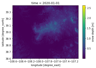
We can make a quick matplotlib-based plot for the subsetted data using the .plot() function supplied by xarray.Dataset objects. For this example, we’ll select one day and plot it:
# simple matplotlilb plot
snd_GM_wy2020_ds.sel(time='2020-01-01').plot();
Similarly we can make an interactive plot using the hvplot accessor and specifying a quadmesh plot type:
# hvplot based map
snd_GM_20200101_plot = snd_GM_wy2020_ds.sel(time='2020-01-01').hvplot.quadmesh(geo=True, rasterize=True, project=True,
xlabel='lon', ylabel='lat', cmap='viridis',
tiles='EsriImagery')
snd_GM_20200101_plot
Pan, zoom, and scroll around the map. Hover over the LIS-SnowModel data to see the data values.
If we try to plot more than one time-step hvplot will also provide a time-slider we can use to scrub back and forth in time:
Note: the time-slider below will only work running in Jupyter Lab (not on the snowex website)
snd_GM_wy2020_ds.sel(time='2020-01').hvplot.quadmesh(geo=True, rasterize=True, project=True,
xlabel='lon', ylabel='lat', cmap='viridis',
tiles='EsriImagery')
From here on out we will stick with hvplot for plotting.
Timeseries Plots
We can generate a timeseries for a given grid cell by selecting and calling the plot function:
# define point to take timeseries (note: must be present in coordinates of dataset)
ts_lon, ts_lat = (-107.8702, 39.0504)
# plot timeseries
snd_GM_wy2020_ds_tc.sel(lat=ts_lat, lon=ts_lon).hvplot.line(title=f'Snow Depth Timeseries @ Lon: {ts_lon}, Lat: {ts_lat}',
xlabel='Date', ylabel='Snow Depth (m)') + \
snd_GM_20200101_plot * gv.Points([(ts_lon, ts_lat)]).opts(size=10, color='red')
In the next section we’ll learn how to create a timeseries over a broader area.
Aggregation
We can perform aggregation operations on the dataset such as min(), max(), mean(), and sum() by specifying the dimensions along which to perform the calculation.
For example we can calculate the daily mean snow depth for the region around Grand Mesa for water year 2020:
Area Average
# take area-averaged mean at each timestep
mean_snd_GM_wy2020_ds = snd_GM_wy2020_ds_tc.mean(['lat', 'lon'])
# inspect the dataset
mean_snd_GM_wy2020_ds
<xarray.DataArray 'SM_SnowDepth_inst' (time: 366)> dask.array<mean_agg-aggregate, shape=(366,), dtype=float32, chunksize=(100,), chunktype=numpy.ndarray> Coordinates: * time (time) datetime64[ns] 2019-10-01 2019-10-02 ... 2020-09-30
# plot timeseries (hvplot knows how to plot based on dataset's dimensionality!)
mean_snd_GM_wy2020_ds.hvplot(title='Mean LIS-SnowModel Snow Depth for Grand Mesa area', xlabel='Date', ylabel='Snow Depth (m)')
Comparing Model Output
Now that we’re familiar with the model output, let’s compare it to two other datasets: SNODAS (raster) and SNOTEL (point).
LIS-SnowModel (raster) vs. SNODAS (raster)
First, we’ll load the SNODAS dataset which we also have hosted on S3 as a Zarr store. This command will take a minute or two to run.
# load SNODAS dataset
#snodas depth
key = "SNODAS/snodas_snowdepth_20161001_20200930.zarr"
snodas_depth_ds = xr.open_zarr(s3.get_mapper(f"{bucket_name}/{key}"), consolidated=True)
# apply scale factor to convert to meters (0.001 per SNODAS user guide)
snodas_depth_ds = snodas_depth_ds * 0.001
Next we define a helper function to extract the (lon, lat) of the nearest grid cell to a given point:
def nearest_grid(ds, pt):
"""
Returns the nearest lon and lat to pt in a given Dataset (ds).
pt : input point, tuple (longitude, latitude)
output:
lon, lat
"""
if all(coord in list(ds.coords) for coord in ['lat', 'lon']):
df_loc = ds[['lon', 'lat']].to_dataframe().reset_index()
else:
df_loc = ds[['orig_lon', 'orig_lat']].isel(time=0).to_dataframe().reset_index()
loc_valid = df_loc.dropna()
pts = loc_valid[['lon', 'lat']].to_numpy()
idx = distance.cdist([pt], pts).argmin()
return loc_valid['lon'].iloc[idx], loc_valid['lat'].iloc[idx]
The next cell will look pretty similar to what we did earlier to plot a timeseries of a single point in the LIS-SnowModel data. The general steps are:
Extract the coordinates of the SNODAS grid cell nearest to our LIS-SnowModel grid cell (
ts_lonandts_latfrom earlier)Subset the SNODAS and LIS-SnowModel data to the grid cells and date ranges of interest
Create the plots!
# drop off irrelevant variables
drop_vars = ['orig_lat', 'orig_lon']
lis_output_ds = lis_output_ds.drop(drop_vars)
# get lon, lat of snodas grid cell nearest to the LIS coordinates we used earlier
snodas_ts_lon, snodas_ts_lat = nearest_grid(snodas_depth_ds, (ts_lon, ts_lat))
# define a date range to plot (shorter = quicker for demo)
start_date, end_date = ('2020-01-01', '2020-06-01')
plot_daterange = slice(start_date, end_date)
# select SNODAS grid cell and subset to plot_daterange
snodas_snd_subset_ds = snodas_depth_ds.sel(lon=snodas_ts_lon,
lat=snodas_ts_lat,
time=plot_daterange)
# select LIS grid cell and subset to plot_daterange
lis_snd_subset_ds = lis_output_ds['SM_SnowDepth_inst'].sel(lat=ts_lat,
lon=ts_lon,
time=plot_daterange)
# create SNODAS snow depth plot
snodas_snd_plot = snodas_snd_subset_ds.hvplot(label='SNODAS')
# create LIS snow depth plot
lis_snd_plot = lis_snd_subset_ds.hvplot(label='LIS-SnowModel')
# create SNODAS vs LIS snow depth plot
lis_vs_snodas_snd_plot = (lis_snd_plot * snodas_snd_plot)
# display the plot
lis_vs_snodas_snd_plot.opts(title=f'Snow Depth @ Lon: {ts_lon}, Lat: {ts_lat}',
legend_position='right',
xlabel='Date',
ylabel='Snow Depth (m)')
LIS-SnowModel (raster) vs. SNODAS (raster) vs. SNOTEL (point)
Now let’s add SNOTEL point data to our plot.
First, we’re going to define some helper functions to load the SNOTEL data:
# load csv containing metadata for SNOTEL sites in a given state (e.g,. 'colorado')
def load_site(state):
# define the path to the file
key = f"SNOTEL/snotel_{state}.csv"
# load the csv into a pandas DataFrame
df = pd.read_csv(s3.open(f's3://{bucket_name}/{key}', mode='r'))
return df
# load SNOTEL data for a specific site
def load_snotel_txt(state, var):
# define the path to the file
key = f"SNOTEL/snotel_{state}{var}_20162020.txt"
# determine how many lines to skip in the file (they start with #)
fh = s3.open(f"{bucket_name}/{key}")
lines = fh.readlines()
skips = sum(1 for ln in lines if ln.decode('ascii').startswith('#'))
# load the data into a pandas DataFrame
df = pd.read_csv(s3.open(f"s3://{bucket_name}/{key}"), skiprows=skips)
# convert the Date column from strings to datetime objects
df['Date'] = pd.to_datetime(df['Date'])
return df
For the purposes of this tutorial let’s load the SNOTEL data for sites in Colorado. We’ll pick one site to plot in a few cells.
# load SNOTEL snow depth for Colorado into a dictionary
snotel_depth = {'CO': load_snotel_txt('CO', 'depth')}
We’ll need another helper function to load the depth data:
# get snotel depth
def get_depth(state, site, start_date, end_date):
# grab the depth for the given state (e.g., CO)
df = snotel_depth[state]
# define a date range mask
mask = (df['Date'] >= start_date) & (df['Date'] <= end_date)
# use mask to subset between time range
df = df.loc[mask]
# extract timeseries for the given site
return pd.concat([df.Date, df.filter(like=site)], axis=1).set_index('Date')
Load the site metadata for Colorado:
co_sites = load_site('colorado')
# peek at the first 5 rows
co_sites.head()
| ntwk | state | site_name | ts | lat | lon | elev | |
|---|---|---|---|---|---|---|---|
| 0 | SNTL | CO | Apishapa (303) | NaN | 37.33 | -105.07 | 10000 |
| 1 | SNTL | CO | Arapaho Ridge (1030) | NaN | 40.35 | -106.35 | 10960 |
| 2 | SNTL | CO | Bear Lake (322) | NaN | 40.31 | -105.65 | 9500 |
| 3 | SNTL | CO | Bear River (1061) | NaN | 40.06 | -107.01 | 9080 |
| 4 | SNTL | CO | Beartown (327) | NaN | 37.71 | -107.51 | 11600 |
The point we’ve been using so far in the tutorial actually corresponds to the coordinates for the Park Reservoir SNOTEL on Grand Mesa! Let’s extract the site data for that point:
# get the depth data by passing the site name to the get_depth() function
park_res_snd_df = get_depth('CO', 'Park Reservoir (682)', start_date, end_date)
# convert from cm to m
park_res_snd_df = park_res_snd_df / 100
Now we’re ready to plot:
# create SNOTEL plot
park_res_plot = park_res_snd_df.hvplot(label='SNOTEL')
# combine the SNOTEl plot with the LIS vs SNODAS plot
(lis_vs_snodas_snd_plot * park_res_plot).opts(title=f'Snow Depth @ Lon: {ts_lon}, Lat: {ts_lat}', legend_position='right')
Interactive Data Exploration
Note:You must run the following code in JupyterLab for interactivity
We’ve now built up the separate pieces for visualizing LIS-SnowModel output spatially and temporally, and we’ve combined our time series with those from SNOTEL stations and SNODAS. Now we can bring it all together in an interactive tool.
The code in the cells below will generate an interactive panel for comparing of LIS-SnowModel output, SNODAS, and SNOTEL snow depth and snow water equivalent at SNOTEL site locations.
Note: some cells below take several minutes to run and some aspects of the interactive widgets may not work in the rendered version on the Hackweek site.
Load Data
SNOTEL Sites info
# create dictionary linking state names and abbreviations
snotel = {"CO" : "colorado",
"ID" : "idaho",
"NM" : "newmexico",
"UT" : "utah",
"WY" : "wyoming"}
# load SNOTEL site metadata for sites in the given state
def load_site(state):
# define path to file
key = f"SNOTEL/snotel_{state}.csv"
# load csv into pandas DataFrame
df = pd.read_csv(s3.open(f'{bucket_name}/{key}', mode='r'))
return df
SNOTEL Depth & SWE
def load_snotel_txt(state, var):
# define path to file
key = f"SNOTEL/snotel_{state}{var}_20162020.txt"
# open text file
fh = s3.open(f"{bucket_name}/{key}")
# read each line and note those that begin with '#'
lines = fh.readlines()
skips = sum(1 for ln in lines if ln.decode('ascii').startswith('#'))
# load txt file into pandas DataFrame (skipping lines beginning with '#')
df = pd.read_csv(s3.open(f"{bucket_name}/{key}"), skiprows=skips)
# convert Date column from str to pandas datetime objects
df['Date'] = pd.to_datetime(df['Date'])
return df
# load SNOTEL depth & swe into dictionaries
# define empty dicts
snotel_depth = {}
snotel_swe = {}
# loop over states and load SNOTEL data
for state in snotel.keys():
print(f"Loading state {state}")
snotel_depth[state] = load_snotel_txt(state, 'depth')
snotel_swe[state] = load_snotel_txt(state, 'swe')
Loading state CO
Loading state ID
Loading state NM
Loading state UT
Loading state WY
SNODAS SWE
We’ve already loaded in SNODAS snow depths, but here we’ll load in SWE. As above, this cell might take a few minutes to run since it’s a large dataset to read.
# load snodas swe data
key = "SNODAS/snodas_swe_20161001_20200930.zarr"
snodas_swe_ds = xr.open_zarr(s3.get_mapper(f"{bucket_name}/{key}"), consolidated=True)
LIS-SnowModel Outputs
We’ve already read in the LIS-SnowModel data above. Here we subset by time for October 2019 - June 2020.
# subset LIS data for winter 2020
time_range = slice('2019-10-01', '2020-06-30')
lis_sf = lis_output_ds_tc.sel(time=time_range)
lis_sf = lis_sf.drop(drop_vars)
In the next cell, we extract the data variable names and timesteps from the LIS outputs. These will be used to define the widget options.
# gather metadata from LIS
# get variable names:string
vnames = list(lis_sf.data_vars)
print(vnames)
# get time-stamps:string
tstamps = list(np.datetime_as_string(lis_sf.time.values, 'D'))
print(len(tstamps), tstamps[0], tstamps[-1])
['SM_SWE_inst', 'SM_SnowDensity_inst', 'SM_SnowDepth_inst']
274 2019-10-01 2020-06-30
By default, the holoviews plotting library automatically adjusts the range of plot colorbars based on the range of values in the data being plotted. This may not be ideal when comparing data on different timesteps. In the next cell we assign the upper and lower bounds for each data variable which we’ll later use to set a static colorbar range.
cmap_lims = {'SM_SWE_inst': (0.0, 3.0),
'SM_SnowDensity_inst': (100, 550.0),
'SM_SnowDepth_inst': (0.0, 6.5)}
Interactive Widget
SNOTEL Site Map and Timeseries
The two cells that follow will create an interactive panel for comparing LIS-SnowModel, SNODAS, and SNOTEL snow depth and snow water equivalent. The SNOTEL site locations are plotted as points on an interactive map for each state. Hover over the sites to view metadata and click on a site to generate a timeseries!
Note: it will take some time for the timeseries to display.
# get snotel depth
def get_depth(state, site, ts, te):
df = snotel_depth[state]
# subset between time range
mask = (df['Date'] >= ts) & (df['Date'] <= te)
df = df.loc[mask]
# extract timeseries for the site
return pd.concat([df.Date, df.filter(like=site)], axis=1).set_index('Date')
# get snotel swe
def get_swe(state, site, ts, te):
df = snotel_swe[state]
# subset between time range
mask = (df['Date'] >= ts) & (df['Date'] <= te)
df = df.loc[mask]
# extract timeseries for the site
return pd.concat([df.Date, df.filter(like=site)], axis=1).set_index('Date')
# co-locate site & LIS-SnowModel model cell
def nearest_grid(pt):
# pt : input point, tuple (longtitude, latitude)
# output:
# x_idx, y_idx
loc_valid = df_loc.dropna()
pts = loc_valid[['lon', 'lat']].to_numpy()
idx = distance.cdist([pt], pts).argmin()
return loc_valid['east_west'].iloc[idx], loc_valid['north_south'].iloc[idx]
# get LIS-SnowModel variable
def var_subset(dset, v, lon, lat, ts, te):
return dset[v].sel(lon=lon, lat=lat, method="nearest").sel(time=slice(ts, te)).load()
# line plots
def line_callback(index, state, vname, ts_tag, te_tag):
sites = load_site(snotel[state])
row = sites.iloc[1]
tmp = var_subset(lis_sf, vname, row.lon, row.lat, ts_tag, te_tag)
xr_sf = xr.zeros_like(tmp)
xr_snodas = xr_sf
ck = get_depth(state, row.site_name, ts_tag, te_tag).to_xarray().rename({'Date': 'time'})
xr_snotel = xr.zeros_like(ck)
if not index:
title='Var: -- Lon: -- Lat: --'
return (xr_sf.hvplot(title=title, color='blue', label='LIS-SnowModel') \
* xr_snotel.hvplot(color='red', label='SNOTEL') \
* xr_snodas.hvplot(color='green', label='SNODAS')).opts(legend_position='right')
else:
sites = load_site(snotel[state])
first_index = index[0]
row = sites.iloc[first_index]
xr_sf = var_subset(lis_sf, vname, row.lon, row.lat, ts_tag, te_tag)
vs = vname.split('_')[1]
title=f'Var: {vs} Lon: {row.lon} Lat: {row.lat}'
# update snotel data
if 'depth' in vname.lower():
xr_snotel = get_depth(state, row.site_name, ts_tag, te_tag).to_xarray().rename({'Date': 'time'})*0.01
xr_snodas = var_subset(snodas_depth_ds, 'SNOWDEPTH', row.lon, row.lat, ts_tag, te_tag)
if 'swe' in vname.lower():
xr_snotel = get_swe(state, row.site_name, ts_tag, te_tag).to_xarray().rename({'Date': 'time'})/1000
xr_snodas = var_subset(snodas_swe_ds, 'SWE', row.lon, row.lat, ts_tag, te_tag)/1000
return xr_sf.hvplot(title=title, color='blue', label='LIS-SnowModel') \
* xr_snotel.hvplot(color='red', label='SNOTEL') \
* xr_snodas.hvplot(color='green', label='SNODAS')
# satic snowdepth as background
dds = lis_sf['SM_SnowDepth_inst'].sel(time='2020-02-01').load()
# prepare the panel that will display a static plot of snow depth. Snotel sites will be plotted on top
img = dds.hvplot.quadmesh(geo=True, rasterize=True, project=True,
xlabel='lon', ylabel='lat', cmap='viridis',
clim=(0,1))
snow_depth_bg=hd.regrid(img)
# sites on map
def plot_points(state):
# dataframe to hvplot obj Points
sites=load_site(snotel[state])
pts_opts=dict(size=10, nonselection_alpha=0.5,tools=['tap', 'hover'])
#site_points=sites.hvplot.points(x='lon', y='lat', c='elev', cmap='fire', geo=True, hover_cols=['site_name', 'ntwk', 'state', 'lon', 'lat']).opts(**pts_opts)
site_points=sites.hvplot.points(x='lon', y='lat', color='black',geo=True, hover_cols=['site_name', 'ntwk', 'state', 'lon', 'lat']).opts(**pts_opts)
return site_points
# base map
tiles = gvts.OSM()
# state widget
state_select = pn.widgets.Select(options=list(snotel.keys()), name="State")
state_stream = Params(state_select, ['value'], rename={'value':'state'})
# variable widget
var_select = pn.widgets.Select(options=['SM_SnowDepth_inst', 'SM_SWE_inst'], name="LIS Variable List")
var_stream = Params(var_select, ['value'], rename={'value':'vname'})
# date range widget
date_fmt = '%Y-%m-%d'
sdate_input = pn.widgets.DatetimeInput(name='Start date', value=dt(2019,10,1),start=dt.strptime(tstamps[0], date_fmt), end=dt.strptime(tstamps[-1], date_fmt), format=date_fmt)
sdate_stream = Params(sdate_input, ['value'], rename={'value':'ts_tag'})
edate_input = pn.widgets.DatetimeInput(name='End date', value=dt(2020,6,30),start=dt.strptime(tstamps[0], date_fmt), end=dt.strptime(tstamps[-1], date_fmt),format=date_fmt)
edate_stream = Params(edate_input, ['value'], rename={'value':'te_tag'})
# generate site points as dynamic map
# plots points and calls plot_points() when user selects a site
site_dmap = hv.DynamicMap(plot_points, streams=[state_stream]).opts(height=400, width=600)
# pick site
select_stream = Selection1D(source=site_dmap)
# link widgets to callback function
line = hv.DynamicMap(line_callback, streams=[select_stream, state_stream, var_stream, sdate_stream, edate_stream])
# create panel layout
pn.Row(snow_depth_bg*site_dmap*tiles, pn.Column(state_select, var_select, pn.Row(sdate_input, edate_input), line))
Exercises
You now know how to see what variables are available in a typical model output file and you’ve learned how to inspect gridded model estimates both spatially and temporally. Below are a few exercises for both practicing the above skills and for becoming more familiar with the sample model output.
Exercise 1
So far we’ve mostly worked with the Grand Mesa region. Can you spatially subset the data to inspect the LIS-SnowModel estimates for the Front Range? What about for Senator Beck basin? Try to use hvplot to plot a map of SWE values for February 2020.
Exercise 2
Here we focused on water year 2020. Can you select a point (maybe the same Park Reservoir SNOTEL point we worked with here) and make a multi-year time series?
Exercise 3 (for an extra challenge!)
We learned about the SnowEx database in a tutorial earlier this week. Can you create a new notebook for combining the model output with your choice of field observation available in the database? Does the model over or underestimate the SnowEx observation?
Conclusion
We’re now more familiar with model output and how to interact with it in Python. The code in this notebook is a great jumping off point for developing more advanced comparisons and interactive widgets.
The Python code can be adapted to other LIS simulations and to other model output as well, with minor modifications. Anyone interested in testing your new skills can combine what you learned here with the other SnowEx Hackweek tutorials - try comparing the LIS-SnowModel output with other snow observations collected during the 2017 field campaign!
For more information on NASA’s Land Information System please see the links below
Resources
Links
References
Kumar, S.V., C.D. Peters-Lidard, Y. Tian, P.R. Houser, J. Geiger, S. Olden, L. Lighty, J.L. Eastman, B. Doty, P. Dirmeyer, J. Adams, K. Mitchell, E. F. Wood, and J. Sheffield, 2006: Land Information System - An interoperable framework for high resolution land surface modeling. Environ. Modeling & Software, 21, 1402-1415, doi:10.1016/j.envsoft.2005.07.004
Peters-Lidard, C.D., P.R. Houser, Y. Tian, S.V. Kumar, J. Geiger, S. Olden, L. Lighty, B. Doty, P. Dirmeyer, J. Adams, K. Mitchell, E.F. Wood, and J. Sheffield, 2007: High-performance Earth system modeling with NASA/GSFC’s Land Information System. Innovations in Systems and Software Engineering, 3(3), 157-165, doi:10.1007/s11334-007-0028-x