SWESARR Tutorial
Contents
SWESARR Tutorial
![]()

- Introduce SWESARR
- Briefly introduce active and passive microwave remote sensing
- Learn how to access, filter, and visualize SWESARR data
Quick References
What is SWESARR?
- Description from Batuhan Osmanoglu.
- Airborne sensor system measuring active and passive microwave measurements
- Colocated measurements are taken simultaneously using an ultra-wideband antenna
SWESARR gives us insights on the different ways active and passive signals are influenced by snow over large areas.
Active and Passive? Microwave Remote Sensing?
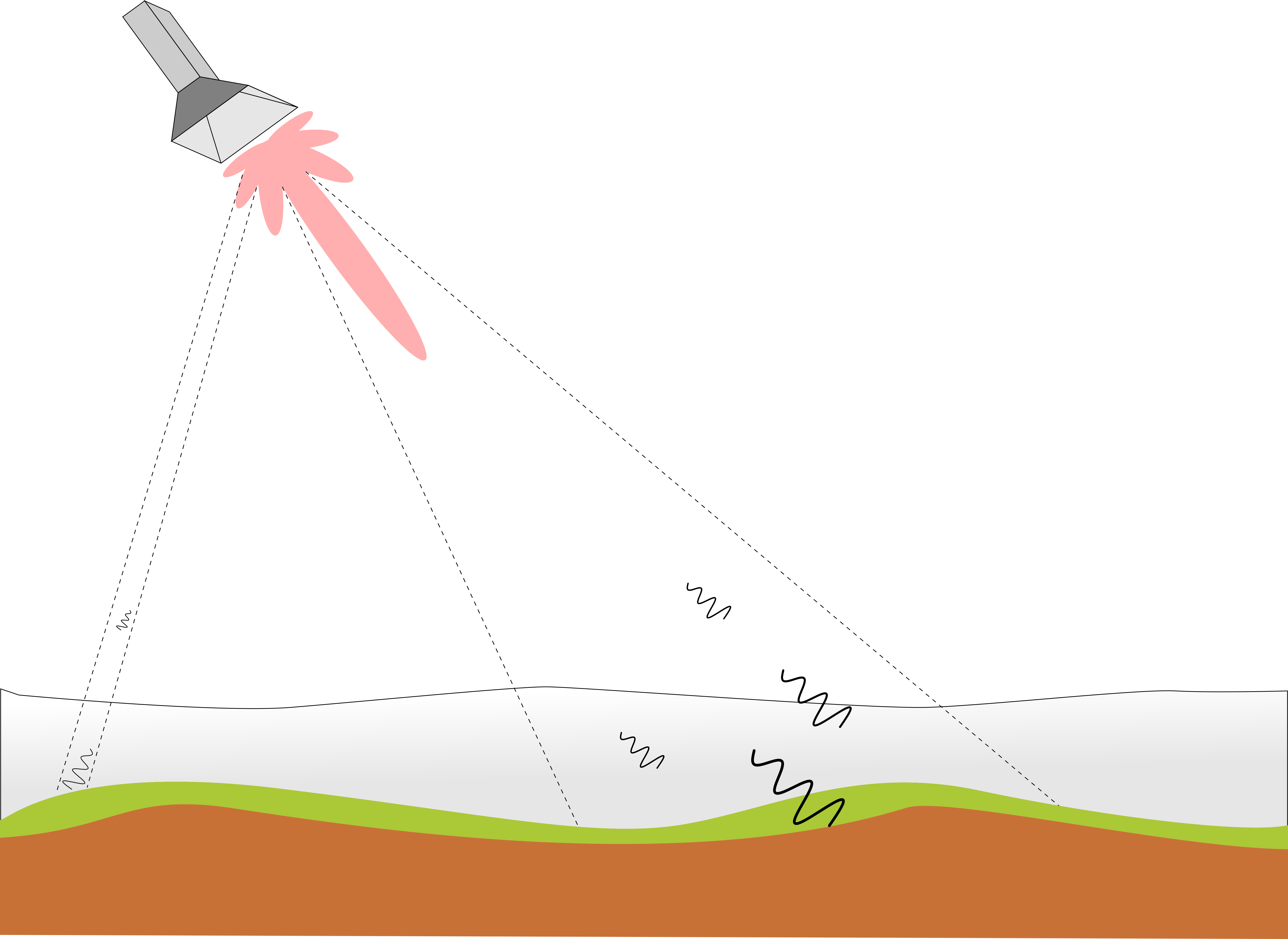
Passive Systems
All materials can naturally emit electromagnetic waves
What is the cause?

Material above zero Kelvin will display some vibration or movement of particles
These moving, charged particles will induce electromagnetic waves
If we’re careful, we can measure these waves with a radio wave measuring tool, or “radiometer”
Radiometers see emissions from many sources, but they’re usually very weak
It’s important to design a radiometer that (1) minimizes side lobes and (2) allows for averaging over the main beam
For this reason, radiometers often have low spatial resolution
✏️ Radiometers allow us to study earth materials through incoherent averaging of naturally emitted signals
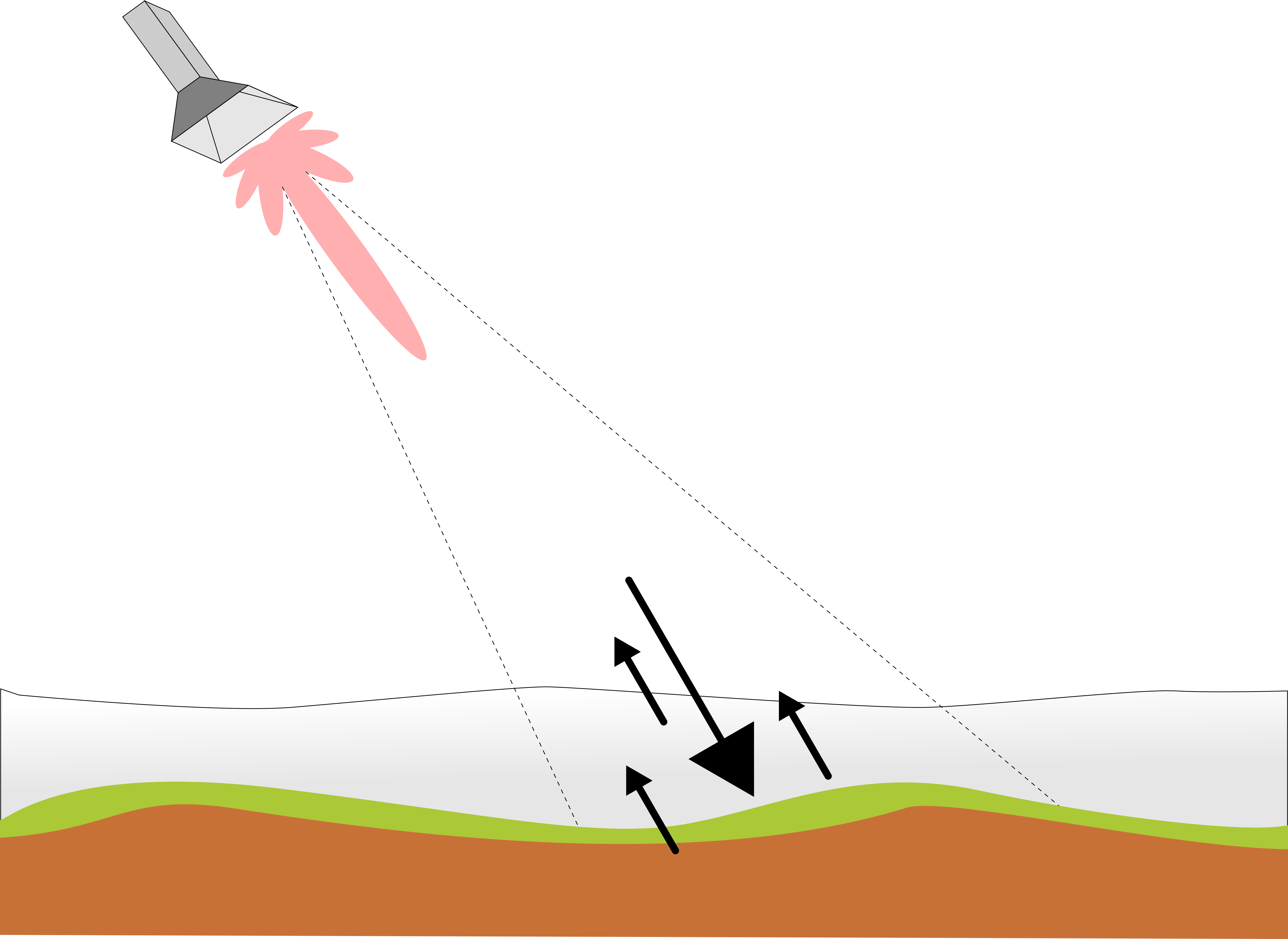
Active Systems
While radiometers generally measure natural electromagnetic waves, radars measure man-made electromagnetic waves
Transmit your own wave, and listen for the returns
The return of this signal is dependent on the surface and volume characteristics of the material it contacts
✏️ Synthetic aperture radar allows for high spatial resolution through processing of coherent signals
%%HTML
<style>
td { font-size: 15px }
th { font-size: 15px }
</style>
SWESARR Sensors
SWESARR Frequencies, Polarization, and Bandwidth Specification
Center-Frequency (GHz) |
Band |
Sensor |
Bandwidth (MHz) |
Polarization |
|---|---|---|---|---|
9.65 |
X |
SAR |
200 |
VH and VV |
10.65 |
X |
Radiometer |
200 |
H |
13.6 |
Ku |
SAR |
200 |
VH and VV |
17.25 |
Ku |
SAR |
200 |
VH and VV |
18.7 |
K |
Radiometer |
200 |
H |
36.5 |
Ka |
Radiometer |
1,000 |
H |


SWESARR Coverage
Below: radiometer coverage for all passes made between February 10 to February 12, 2020
SWESARR flights cover many snowpit locations over the Grand Mesa area as shown by the dots in blue

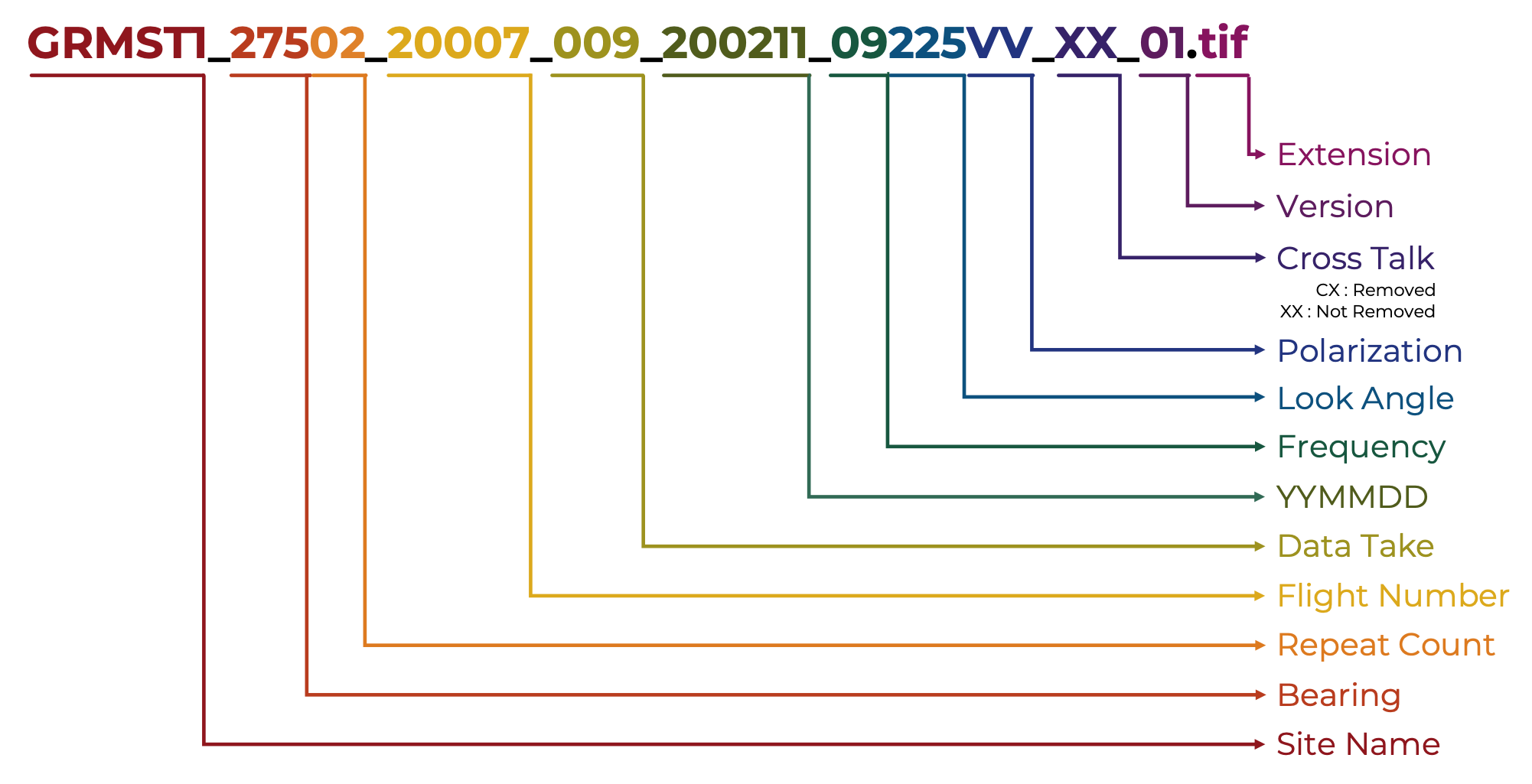
Reading SWESARR Data
SWESARR’s SAR data is organized with a common file naming convention for finding the time, location, and type of data
Accessing Data: SAR
SAR Data Example
# Import several libraries.
# comments to the right could be useful for local installation on Windows.

from shapely import speedups      # https://www.lfd.uci.edu/~gohlke/pythonlibs/
speedups.disable()                # <-- handle a potential error in cartopy

import requests                   # !conda install -c anaconda requests

# raster manipulation libraries
import rasterio                   # https://www.lfd.uci.edu/~gohlke/pythonlibs/
from osgeo import gdal            # https://www.lfd.uci.edu/~gohlke/pythonlibs/
import cartopy.crs as ccrs        # https://www.lfd.uci.edu/~gohlke/pythonlibs/
import rioxarray as rxr           # !conda install -c conda-forge rioxarray
import xarray as xr               # !conda install -c conda-forge xarray dask netCDF4 bottleneck

# plotting tools
from matplotlib import pyplot     # !conda install matplotlib
import datashader as ds           # https://www.lfd.uci.edu/~gohlke/pythonlibs/
import hvplot.xarray              # !conda install hvplot

# append the subfolders of the current working directory to pythons path

import os
import sys

swesarr_subdirs = ["data", "util"]
tmp = [sys.path.append(os.getcwd() + "/" + sd) for sd in swesarr_subdirs]
del tmp # suppress Jupyter notebook output, delete variable

from helper import gdal_corners, join_files, join_sar_radiom
Select your data
# select files to download

# SWESARR data website
source_repo = 'https://glihtdata.gsfc.nasa.gov/files/radar/SWESARR/prerelease/'

# Example flight line
flight_line = 'GRMCT2_31801_20007_016_200211_225_XX_01/'

# SAR files within this folder
data_files = [
    'GRMCT2_31801_20007_016_200211_09225VV_XX_01.tif',
    'GRMCT2_31801_20007_016_200211_09225VH_XX_01.tif',
    'GRMCT2_31801_20007_016_200211_13225VV_XX_01.tif',
    'GRMCT2_31801_20007_016_200211_13225VH_XX_01.tif',
    'GRMCT2_31801_20007_016_200211_17225VV_XX_01.tif',
    'GRMCT2_31801_20007_016_200211_17225VH_XX_01.tif'
]

# store the location of the SAR tiles as they're located on the SWESARR data server
remote_tiles = [source_repo + flight_line + d for d in data_files]

# create local output data directory
output_dir = os.getcwd() + '/data/'
try:
    os.makedirs(output_dir)
except FileExistsError:
    print('output directory prepared!')

# store individual TIF files locally on our computer / server
output_paths = [output_dir + d for d in data_files]
output directory prepared!
Download SAR data and place into data folder
##    for each file selected, store the data locally
##
##    only run this block if you want to store data on the current
##    server/hard drive this notebook is located.
##
################################################################

for remote_tile, output_path in zip(remote_tiles, output_paths):

    # download data
    r = requests.get(remote_tile)

    # Store data (~= 65 MB/file)
    if r.status_code == 200:
        with open(output_path, 'wb') as f:
            f.write(r.content)
Merge SAR datasets into single xarray file
da = join_files(output_paths)
da
<xarray.DataArray (band: 6, y: 4289, x: 3959)>
dask.array<concatenate, shape=(6, 4289, 3959), dtype=float32, chunksize=(1, 1200, 1200), chunktype=numpy.ndarray>
Coordinates:
  * band         (band) <U4 '09VV' '09VH' '13VV' '13VH' '17VV' '17VH'
  * x            (x) float64 7.396e+05 7.396e+05 ... 7.475e+05 7.475e+05
  * y            (y) float64 4.329e+06 4.329e+06 4.329e+06 ... 4.32e+06 4.32e+06
    spatial_ref  int64 0
Attributes:
    _FillValue:    nan
    scale_factor:  1.0
add_offset: 0.0Plot data with hvplot
# Set clim directly:
clim=(-20,20)
cmap='gray'
crs = ccrs.UTM(zone='12') #12n
tiles='OSM'
tiles='EsriImagery'

da.hvplot.image(x='x',y='y',groupby='band',cmap=cmap,clim=clim,rasterize=True,
                       xlabel='Longitude',ylabel='Latitude',
                       frame_height=500, frame_width=500,
                       xformatter='%.1f',yformatter='%.1f', crs=crs, tiles=tiles, alpha=0.8)
🎉 Congratulations! You now know how to download and display a SWESARR SAR dataset !
Radiometer Data Example
SWESARR’s radiometer data is publicly available at NSIDC
Will be available on SnowExSQL if the fans demand it!
import pandas as pd      # !conda install pandas
import numpy as np       # !conda install numpy
import xarray as xr      # !conda install -c anaconda xarray

import hvplot            # !conda install hvplot
import hvplot.pandas
import holoviews as hv   # !conda install -c conda-forge holoviews
from holoviews.operation.datashader import datashade
from geopy.distance import distance     #!conda install -c conda-forge geopy
Downloading SWESARR Radiometer Data with wget
If you are running this on the SnowEx Hackweek server,
wgetshould be configured.If you are using this tutorial on your local machine, you’ll need
wget.Linux Users
You should be fine. This is likely baked into your operating systems. Congratulations! You chose correctly.
Apple Users
The author of this textbox has never used a Mac. There are many command-line suggestions online.
sudo brew install wget,sudo port install wget, etc. Try searching online!
Windows Users
Check out this tutorial, page 2 You’ll need to download binaries for
wget, and you should really make it an environment variable!
Be sure to be diligent before installing anything to your computer.
Regardless, fill in your NASA Earthdata Login credentials and follow along!
# !wget --user=USERNAME_HERE --password=PASSWORD_HERE --quiet https://n5eil01u.ecs.nsidc.org/SNOWEX/SNEX20_SWESARR_TB.001/2020.02.12/SNEX20_SWESARR_TB_GRMCT2_13801_20007_000_200211_XKKa225H_v01.csv -O {output_dir}/SNEX20_SWESARR_TB_GRMCT2_13801_20007_000_200211_XKKa225H_v01.csv
# !wget --quiet https://n5eil01u.ecs.nsidc.org/SNOWEX/SNEX20_SWESARR_TB.001/2020.02.12/SNEX20_SWESARR_TB_GRMCT2_13801_20007_000_200211_XKKa225H_v01.csv -O {output_dir}/SNEX20_SWESARR_TB_GRMCT2_13801_20007_000_200211_XKKa225H_v01.csv
Select an example radiometer data file
# use the file we downloaded with wget above
excel_path = f'{output_dir}/SNEX20_SWESARR_TB_GRMCT2_13801_20007_000_200211_XKKa225H_v01.csv'

# read data
radiom = pd.read_csv(excel_path)
Lets examine the radiometer data files content
radiom.head()
#radiom.hvplot.table(width=1100) # sortable table in jupyterlab
| UTC | Longitude (deg) | Latitude (deg) | Elevation (m) | TB X (K) | TB K (K) | TB Ka (K) | Antenna Longitude (deg) | Antenna Latitude (deg) | Antenna Altitude (m) | Antenna Yaw (deg) | Antenna Pitch (deg) | Antenna Look Angle (deg) | |
|---|---|---|---|---|---|---|---|---|---|---|---|---|---|
| 0 | 20200211-18:33:53.048360 | -108.227372 | 39.071994 | 2971 | 247.1 | 241.2 | 231.2 | -108.052329 | 38.940324 | 4525.7 | 2.02 | 3.53 | 44.9 |
| 1 | 20200211-18:33:53.148380 | -108.227372 | 39.071901 | 2979 | 246.3 | 238.2 | 229.3 | -108.052331 | 38.940326 | 4525.7 | 2.04 | 3.53 | 44.9 |
| 2 | 20200211-18:33:53.248380 | -108.227372 | 39.071809 | 2979 | 247.8 | 237.5 | 227.4 | -108.052334 | 38.940329 | 4525.7 | 2.06 | 3.53 | 44.9 |
| 3 | 20200211-18:33:53.348380 | -108.227279 | 39.071716 | 2991 | 247.2 | 237.5 | 225.4 | -108.052336 | 38.940331 | 4525.7 | 2.05 | 3.53 | 44.9 |
| 4 | 20200211-18:33:53.448380 | -108.227279 | 39.071716 | 2991 | 245.7 | 237.4 | 222.6 | -108.052339 | 38.940333 | 4525.6 | 2.05 | 3.53 | 44.9 |
Plot radiometer data with hvplot
# create several series from pandas dataframe

lon_ser = pd.Series( radiom['Longitude (deg)'].to_list() * (3) )
lat_ser = pd.Series( radiom['Latitude (deg)'].to_list() * (3) )

tb_ser = pd.Series(
    radiom['TB X (K)'].to_list() + radiom['TB K (K)'].to_list() +
    radiom['TB Ka (K)'].to_list(), name="Tb"
     )

# get series length, create IDs for plotting
sl = len(radiom['TB X (K)'])
id_ser = pd.Series(
    ['X-band']*sl + ['K-band']*sl + ['Ka-band']*sl, name="ID"
     )

frame = {'Longitude (deg)' : lon_ser, 'Latitude (deg)' : lat_ser,
         'TB' : tb_ser, 'ID' : id_ser}
radiom_p = pd.DataFrame(frame)

del sl, lon_ser, lat_ser, tb_ser, id_ser, frame

radiom_p.hvplot.points('Longitude (deg)', 'Latitude (deg)', groupby='ID', geo=True, color='TB', alpha=1,
                        tiles='ESRI', height=400, width=500)
🎉 Congratulations! You now know how to download and display a SWESARR radiometer dataset !
SAR and Radiometer Together
The novelty of SWESARR lies in its colocated SAR and radiometer systems
Lets try filtering the SAR dataset and plotting both datasets together
For this session, I’ve made the code a function. We can look at it together by opening
.util/helper.py
data_p, data_ser = join_sar_radiom(da, radiom)

data_p.hvplot.points('Longitude (deg)', 'Latitude (deg)', groupby='ID', geo=True, color='Measurements', alpha=1,
                        tiles='ESRI', height=400, width=500)
Exercise
- Plot a time-series visualization of the filtered SAR channels from the output of the join_sar_radiom() function
- Plot a time-series visualization of the radiometer channels from the output of the join_sar_radiom() function
- Hint: the data series variable ( data_ser ) is a pandas data series. Use some of the methods shown above to read and plot the data!
### Your Code Here #############################################################################################################
#
# Two of Many Options:
# 1.) Go the matplotlib route
#     a.) Further reading below:
#         https://matplotlib.org/stable/tutorials/introductory/pyplot.html
#
# 2.) Try using hvplot tools if you like
#      a.) Further reading below:
#          https://hvplot.holoviz.org/user_guide/Plotting.html
#
# Remember, if you don't use a library all of the time, you'll end up <search engine of your choice>-ing it. Go crazy!
#
################################################################################################################################

# configure some inline parameters to make things pretty / readable if you'd like to go with matplotlib
%matplotlib inline
import matplotlib.pyplot as plt
plt.rcParams["figure.figsize"] = (16, 9) # (w, h)