Introduction to AVIRIS-NG
Contents
Introduction to AVIRIS-NG

Contributors: Joachim Meyer1, Chelsea Ackroyd1, McKenzie Skiles1, Phil Dennison1, Keely Roth1
1University of Utah
Learning Objectives
Become familiar with hyperspectral data, including data orginiating from AVIRIS-NG
Understand the fundamental methods for displaying and exploring hyperspectral data in Python
Identify the amount of ice in a given pixel using spectral feature fitting methodology
Review of Hyperspectral Data
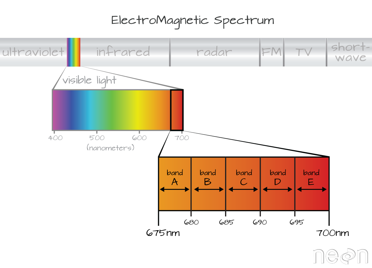
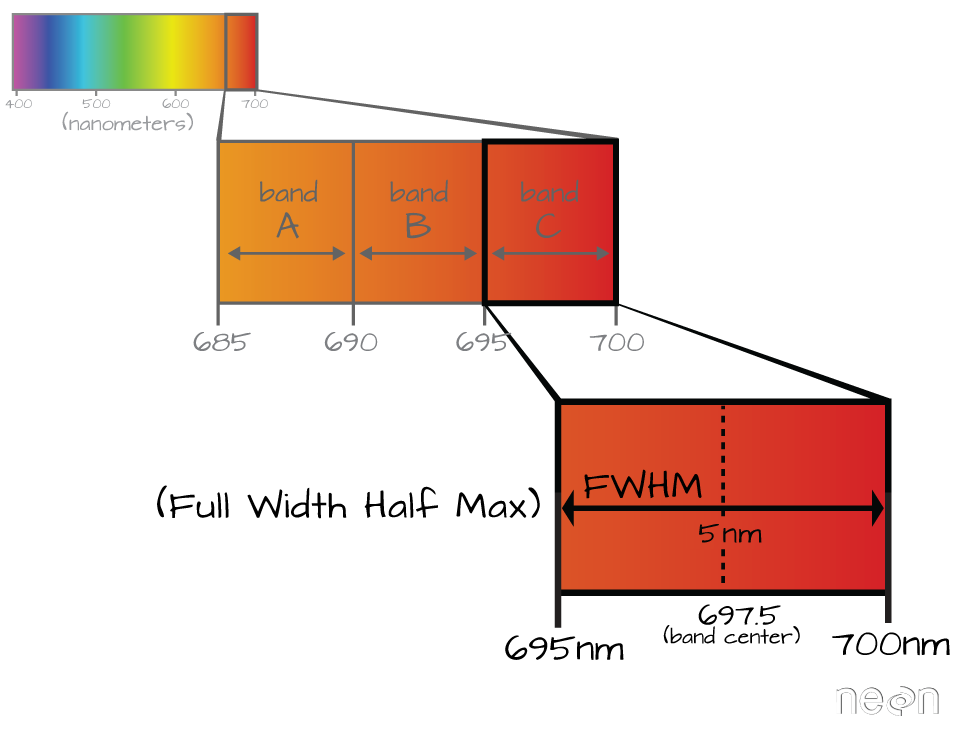
Incoming solar radiation is either reflected, absorbed, or transmitted (or a combination of all three) depending on the surface material. This spectral response allows us to identify varying surface types (e.g. vegetation, snow, water, etc.) in a remote sensing image. The spectral resolution, or the wavelength interval, determines the amount of detail recorded in the spectral response: finer spectral resolutions have bands with narrow wavelength intervals, while coarser spectral resolutions have bands with larger wavelength intervals, and therefore, less detail in the spectral response.
https://www.neonscience.org/resources/learning-hub/tutorials/hyper-spec-intro
Multispectral vs. Hyperspectral Data
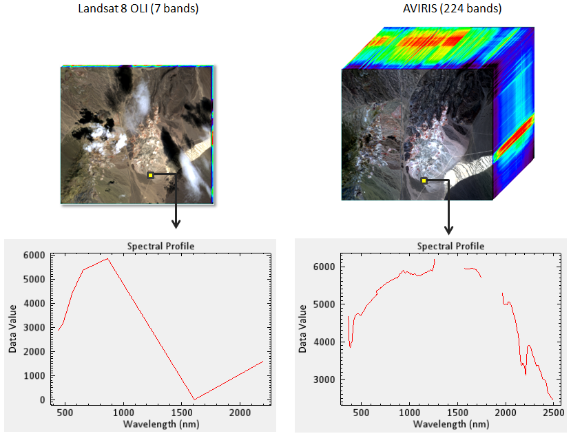
Multispectral instruments have larger spectral resolutions with fewer bands. This level of detail can be limiting in distinguishing between surface types. Hyperspectral instruments, in comparison, typically have hundreds of bands with relatively narrow wavelength intervals. The image below illustrates the difference in spectral responses between a multispectral (Landsat 8 OLI) and a hyperspectral (AVIRIS) sensor.
AVIRIS-NG Meets SnowEx
AVIRIS-NG measures upwelling radiance across 485 continuous spectral bands.
Flight Altitude |
Spatial Resolution |
Spectral Resolution |
Spectral Range |
|---|---|---|---|
25,000 ft ASL |
4 m |
5 nm |
308 nm to 2510 nm |
Flight Dates |
Study Site |
|---|---|
2021-03-19 |
Senator Beck Basin |
2021-03-19 |
Grand Mesa |
2021-04-11 |
Senator Beck Basin |
2021-04-11 |
Grand Mesa |
2021-04-29 |
Senator Beck Basin |
2021-04-29 |
Grand Mesa |
Accessing the data
Data products:
Spectral radiance/observation geometry (L1B)
Corrected Reflectance (L2)
L2 will be available to the public soon via NSIDC
First look at the data
Important
You will always want the data file and the header file when processing.
For today, we are downloading and using a subsample that encompasses Swamp Angel Study Plot. The download is done via the Python urllib.request native library.
import urllib.request
The data file
SBB_data_file = 'data/ang20210411t181022_rfl_v2z1a_img_SASP'
urllib.request.urlretrieve(
    'https://github.com/snowex-hackweek/tutorial-data/blob/main/SnowEx-2022/AVIRIS-NG/ang20210411t181022_rfl_v2z1a_img_SASP?raw=true',
    SBB_data_file
);
The header file
SBB_header_file = 'data/ang20210411t181022_rfl_v2z1a_img_SASP.hdr'
urllib.request.urlretrieve(
    'https://raw.githubusercontent.com/snowex-hackweek/tutorial-data/main/SnowEx-2022/AVIRIS-NG/ang20210411t181022_rfl_v2z1a_img_SASP.hdr',
    SBB_header_file
);
The original header file (hold on tight on why …)
original_header_file = 'data/ang20210411t181022_rfl_v2z1a_img.hdr'
urllib.request.urlretrieve(
    'https://raw.githubusercontent.com/snowex-hackweek/tutorial-data/main/SnowEx-2022/AVIRIS-NG/ang20210411t181022_rfl_v2z1a_img.hdr',
    original_header_file
);
Exploring multiple flight lines
Interactive exploration using GeoPandas and the folium plotting library:
import geopandas
import folium
Create an index
With a little help from GDAL and the gdaltindex command, we can create an index for all flight lines and see where they are:
An example command that creates a GeoPackage
gdaltindex -t_srs EPSG:4326 index.gpkg ang20210411t1*_rfl*img
Breaking down the command:
This command creates an index file index.gpkg for all flight lines starting with ang20210411t1* and selects only the reflectance prodcuts _rfl*img. The star * acts as a wildcard to include more than one file where the elements of the string as whole matches. The -t_srs EPSG:4326 ensures that the read projection for all files will be stored as WGS 84 in the index. It does not change anything with the flight line data itself.
Specifically for hyperspectral data, it is important to not include the header files (ending with .hdr). GDAL automatically reads those with every image file and adding them to the list of files would cause a duplication.
One way to test the included files is to use the search string with the list (ls -lh) command in the terminal.
The -l option lists the output with one line per file, and -h will show file size in ‘human readable’ units such as MB and GB.
Example:
ls -lh index.gpkg ang20210411t1*_rfl*img
Sample output:
-rw-r--r-- username groupname 2.3G Feb 16 08:23 ang20210411t180555_rfl_v2z1a_img
-rw-r--r-- username groupname 1.6G Feb 16 08:24 ang20210411t181022_rfl_v2z1a_img
-rw-r--r-- username groupname 1.9G Feb 16 08:23 ang20210411t181414_rfl_v2z1a_img
-rw-r--r-- username groupname 1.8G Feb 16 08:23 ang20210411t181822_rfl_v2z1a_img
Load the created index and some geospatial information into a GeoDataframe to explore interactively
GeoPandas has the ability to read files from disk or from a remote URL. When using a URL the information is held in memory for that session and will be lost once you restart the Python kernel.
flight_lines = geopandas.read_file('https://github.com/snowex-hackweek/tutorial-data/blob/main/SnowEx-2022/AVIRIS-NG/20210411_flights.gpkg?raw=true')
sbb = geopandas.read_file('https://raw.githubusercontent.com/snowex-hackweek/tutorial-data/main/SnowEx-2022/AVIRIS-NG/SBB_basin.geojson')
swamp_angel = geopandas.read_file('https://raw.githubusercontent.com/snowex-hackweek/tutorial-data/main/SnowEx-2022/AVIRIS-NG/SwampAngel.geojson')
# Create a map with multiple layers to explore where the lines are
## Layer 1 used as base layer
sbb_layer = sbb.explore(
    name='SBB basin',
    color='green'
)
## Layer 2
swamp_angel.explore(
    m=sbb_layer,                   ## Add this layer to the Layer 1
    name='Swamp Angel Study Plot'
)
## Layer 3
flight_lines.explore(
    m=sbb_layer,                   ## Add this layer to the Layer 1
    name='AVIRIS flight lines',
    column='location'
)
# Top right box to toggle layer visibility
folium.LayerControl().add_to(sbb_layer)

# Show the final map with all layer
sbb_layer
Exploring a single flight line
Check our current file location (This is called a magic command)
%pwd
'/home/runner/work/website-2022/website-2022/book/tutorials/aviris-ng'
We can store this output in a local variable
home_folder = %pwd
Create absolute paths to our downloaded files
SBB_data_file = f'{home_folder}/{SBB_data_file}'
SBB_header_file = f'{home_folder}/{SBB_header_file}'
Spectral Python library
import spectral
# Create a file object for the original image
image = spectral.open_image(SBB_header_file)
# Get information about the bands
image.bands.centers
Darn … we have an empty output. This subset was created using the GDAL library. Unfortunately, GDAL does not write the headers in a format that the spectral library recognizes. This is where the original header file comes into play.
import spectral.io.envi as envi
Attention
We are accessing the original header, not the subset data file. This is a workaround to get to the band information
header = envi.open(original_header_file, SBB_data_file)
Find band index for a wavelength
import numpy as np
type(header.bands)
spectral.spectral.BandInfo
Ahhh … much better
bands = np.array(header.bands.centers)
bands
array([ 377.071821,  382.081821,  387.091821,  392.101821,  397.101821,
        402.111821,  407.121821,  412.131821,  417.141821,  422.151821,
        427.161821,  432.171821,  437.171821,  442.181821,  447.191821,
        452.201821,  457.211821,  462.221821,  467.231821,  472.231821,
        477.241821,  482.251821,  487.261821,  492.271821,  497.281821,
        502.291821,  507.301821,  512.301821,  517.311821,  522.321821,
        527.331821,  532.341821,  537.351821,  542.361821,  547.361821,
        552.371821,  557.381821,  562.391821,  567.401821,  572.411821,
        577.421821,  582.431821,  587.431821,  592.441821,  597.451821,
        602.461821,  607.471821,  612.481821,  617.491821,  622.491821,
        627.501821,  632.511821,  637.521821,  642.531821,  647.541821,
        652.551821,  657.561821,  662.561821,  667.571821,  672.581821,
        677.591821,  682.601821,  687.611821,  692.621821,  697.621821,
        702.631821,  707.641821,  712.651821,  717.661821,  722.671821,
        727.681821,  732.691821,  737.691821,  742.701821,  747.711821,
        752.721821,  757.731821,  762.741821,  767.751821,  772.751821,
        777.761821,  782.771821,  787.781821,  792.791821,  797.801821,
        802.811821,  807.821821,  812.821821,  817.831821,  822.841821,
        827.851821,  832.861821,  837.871821,  842.881821,  847.881821,
        852.891821,  857.901821,  862.911821,  867.921821,  872.931821,
        877.941821,  882.951821,  887.951821,  892.961821,  897.971821,
        902.981821,  907.991821,  913.001821,  918.011821,  923.021821,
        928.021821,  933.031821,  938.041821,  943.051821,  948.061821,
        953.071821,  958.081821,  963.081821,  968.091821,  973.101821,
        978.111821,  983.121821,  988.131821,  993.141821,  998.151821,
       1003.151821, 1008.161821, 1013.171821, 1018.181821, 1023.191821,
       1028.201821, 1033.211821, 1038.211821, 1043.221821, 1048.231821,
       1053.241821, 1058.251821, 1063.261821, 1068.271821, 1073.281821,
       1078.281821, 1083.291821, 1088.301821, 1093.311821, 1098.321821,
       1103.331821, 1108.341821, 1113.341821, 1118.351821, 1123.361821,
       1128.371821, 1133.381821, 1138.391821, 1143.401821, 1148.411821,
       1153.411821, 1158.421821, 1163.431821, 1168.441821, 1173.451821,
       1178.461821, 1183.471821, 1188.471821, 1193.481821, 1198.491821,
       1203.501821, 1208.511821, 1213.521821, 1218.531821, 1223.541821,
       1228.541821, 1233.551821, 1238.561821, 1243.571821, 1248.581821,
       1253.591821, 1258.601821, 1263.601821, 1268.611821, 1273.621821,
       1278.631821, 1283.641821, 1288.651821, 1293.661821, 1298.671821,
       1303.671821, 1308.681821, 1313.691821, 1318.701821, 1323.711821,
       1328.721821, 1333.731821, 1338.731821, 1343.741821, 1348.751821,
       1353.761821, 1358.771821, 1363.781821, 1368.791821, 1373.801821,
       1378.801821, 1383.811821, 1388.821821, 1393.831821, 1398.841821,
       1403.851821, 1408.861821, 1413.861821, 1418.871821, 1423.881821,
       1428.891821, 1433.901821, 1438.911821, 1443.921821, 1448.931821,
       1453.931821, 1458.941821, 1463.951821, 1468.961821, 1473.971821,
       1478.981821, 1483.991821, 1488.991821, 1494.001821, 1499.011821,
       1504.021821, 1509.031821, 1514.041821, 1519.051821, 1524.061821,
       1529.061821, 1534.071821, 1539.081821, 1544.091821, 1549.101821,
       1554.111821, 1559.121821, 1564.121821, 1569.131821, 1574.141821,
       1579.151821, 1584.161821, 1589.171821, 1594.181821, 1599.191821,
       1604.191821, 1609.201821, 1614.211821, 1619.221821, 1624.231821,
       1629.241821, 1634.251821, 1639.251821, 1644.261821, 1649.271821,
       1654.281821, 1659.291821, 1664.301821, 1669.311821, 1674.321821,
       1679.321821, 1684.331821, 1689.341821, 1694.351821, 1699.361821,
       1704.371821, 1709.381821, 1714.381821, 1719.391821, 1724.401821,
       1729.411821, 1734.421821, 1739.431821, 1744.441821, 1749.451821,
       1754.451821, 1759.461821, 1764.471821, 1769.481821, 1774.491821,
       1779.501821, 1784.511821, 1789.511821, 1794.521821, 1799.531821,
       1804.541821, 1809.551821, 1814.561821, 1819.571821, 1824.581821,
       1829.581821, 1834.591821, 1839.601821, 1844.611821, 1849.621821,
       1854.631821, 1859.641821, 1864.651821, 1869.651821, 1874.661821,
       1879.671821, 1884.681821, 1889.691821, 1894.701821, 1899.711821,
       1904.711821, 1909.721821, 1914.731821, 1919.741821, 1924.751821,
       1929.761821, 1934.771821, 1939.781821, 1944.781821, 1949.791821,
       1954.801821, 1959.811821, 1964.821821, 1969.831821, 1974.841821,
       1979.841821, 1984.851821, 1989.861821, 1994.871821, 1999.881821,
       2004.891821, 2009.901821, 2014.911821, 2019.911821, 2024.921821,
       2029.931821, 2034.941821, 2039.951821, 2044.961821, 2049.971821,
       2054.971821, 2059.981821, 2064.991821, 2070.001821, 2075.011821,
       2080.021821, 2085.031821, 2090.041821, 2095.041821, 2100.051821,
       2105.061821, 2110.071821, 2115.081821, 2120.091821, 2125.101821,
       2130.101821, 2135.111821, 2140.121821, 2145.131821, 2150.141821,
       2155.151821, 2160.161821, 2165.171821, 2170.171821, 2175.181821,
       2180.191821, 2185.201821, 2190.211821, 2195.221821, 2200.231821,
       2205.231821, 2210.241821, 2215.251821, 2220.261821, 2225.271821,
       2230.281821, 2235.291821, 2240.301821, 2245.301821, 2250.311821,
       2255.321821, 2260.331821, 2265.341821, 2270.351821, 2275.361821,
       2280.361821, 2285.371821, 2290.381821, 2295.391821, 2300.401821,
       2305.411821, 2310.421821, 2315.431821, 2320.431821, 2325.441821,
       2330.451821, 2335.461821, 2340.471821, 2345.481821, 2350.491821,
       2355.491821, 2360.501821, 2365.511821, 2370.521821, 2375.531821,
       2380.541821, 2385.551821, 2390.561821, 2395.561821, 2400.571821,
       2405.581821, 2410.591821, 2415.601821, 2420.611821, 2425.621821,
       2430.621821, 2435.631821, 2440.641821, 2445.651821, 2450.661821,
       2455.671821, 2460.681821, 2465.691821, 2470.691821, 2475.701821,
       2480.711821, 2485.721821, 2490.731821, 2495.741821, 2500.751821])
Inspect spatial metadata
header.metadata['map info']
['UTM',
 '1',
 '1',
 '261034.240288',
 '4202245.79268',
 '4.0',
 '4.0',
 '13',
 'North',
 'WGS-84',
 'units=Meters',
 'rotation=-15.0000000']
The map info has geographic information in the following order:
Projection name
Reference (tie point in x pixel-space)
Reference (tie point in y pixel-space)
Pixel easting (in projection coordinates)
Pixel northing (in projection coordinates)
X resolution in geodetic space
y resolution in geodetic space
Projection zone (when UTM)
North or South (when UTM)
Units (Projection)
Rotation
Exploring the data
Define wavelengths for the colors we want
red = 645
green = 510
blue = 440
np.argmin(np.abs(bands - red))
53
bands[54]
647.541821
Create a method to get the values for many different wavelengths
def index_for_band(band):
    # Return the index with the minimum difference between the target and available band center
    return np.argmin(np.abs(bands - band))
index_for_band(green)
27
index_for_band(blue)
13
Inspection plot for selected bands
import matplotlib.pyplot as plt

%matplotlib inline
#Increase the default figure output resolution
plt.rcParams['figure.dpi'] = 200
Subset of Swamp Angel Study Plot (SASP)
Use GDAL warp to subset
gdalwarp -co INTERLEAVE=BIL -of ENVI \                                   # Preserve the data as ENVI file
         -te 261469.404472 4198850.600453 261811.425717 4199084.295516 \ # The target extent
         ang20210411t181022_rfl_v2z1a_img                                # Source file
         ang20210411t181022_rfl_v2z1a_img_SASP                           # Destination file
Important
Going back to the original header file for the spatial extent
Show some first image information
image = spectral.open_image(SBB_header_file)

print(image)
	Data Source:   '/home/runner/work/website-2022/website-2022/book/tutorials/aviris-ng/data/ang20210411t181022_rfl_v2z1a_img_SASP'
	# Rows:             58
	# Samples:          86
	# Bands:           425
	Interleave:        BIL
	Quantization:  32 bits
	Data format:   float32
# Loads the entire image into memory as an array
image_data = image.load()
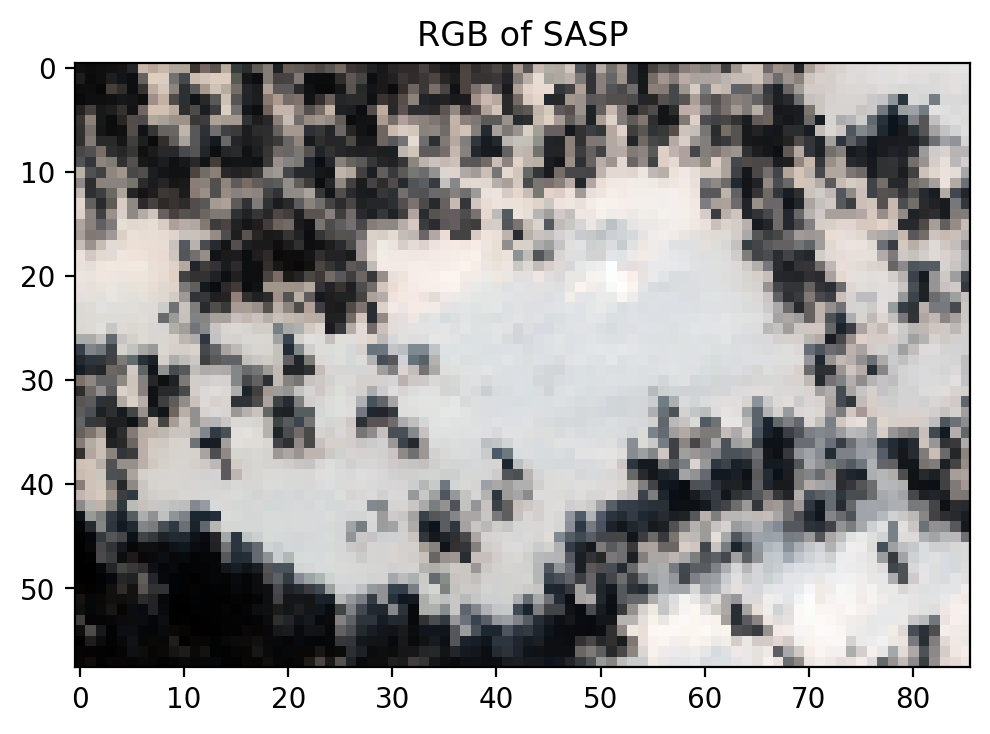
Plot the image based on the previously determined band indices (RGB)
view = spectral.imshow(image_data, (53,27,13), title = 'RGB of SASP')
Exercise
Pick the wavelengths of your choice and plot the Swamp Angel Study plot.
Which bands did you pick? Does the image look as expected?
Let’s discuss the result with your neighbour.
Introduction to Spectral Feature Fitting
Now that we know how to access and explore hyperspectral data, we can take advantage of the detailed spectral signature to better understand the surface characteristics. For instance, using the Spectral Feature Fitting method, we can compare the absorption features within the image spectra to a reference spectra in order to identify the presence of a specific material within a given pixel. Here, we will demonstrate this using the ice absorption feature in a snow-covered pixel found within Swamp Angel Study Plot.
To do so, we will follow the principles of the Beer-Lambert equation, which assumes one-way transmittance through a homogeneous medium:
where \(E_{0\lambda}\) and \(E_\lambda\) are the initial and measured spectral irradiance, respectively, \(\alpha_\lambda\) is a wavelength-specific absorption coefficient, and \(d\) is the distance (i.e. thickness) that absorption occurs over. This will allow us to estimate an “equivalent thickness” of ice in a pixel.
Load the reference spectra
First, we’ll start by loading the reference spectra. This table provides the simple refractive index (\(n_\lambda\)) and the extinction coefficient (\(k_\lambda\)) for water and ice between 400 and 2500 nm.
ref_spectra_fname = 'data/h2o_indices.csv'
urllib.request.urlretrieve(
    'https://raw.githubusercontent.com/snowex-hackweek/tutorial-data/main/SnowEx-2022/AVIRIS-NG/h2o_indices.csv',
    ref_spectra_fname
);
# Read the file into a numpy array
ref_spectra = np.loadtxt(ref_spectra_fname, delimiter=",", skiprows=1)  # Skip the header row

# Let's take a look at the dimensions of our new array and print out the first few and last few lines.
print(ref_spectra.shape)
ref_spectra
(421, 5)
array([[4.00000000e+02, 1.33810000e+00, 1.90000000e-09, 1.31940000e+00,
        2.71000000e-09],
       [4.05000000e+02, 1.33800000e+00, 1.72000000e-09, 1.31900000e+00,
        2.62000000e-09],
       [4.10000000e+02, 1.33790000e+00, 1.59000000e-09, 1.31850000e+00,
        2.51000000e-09],
       ...,
       [2.49000000e+03, 1.26440000e+00, 1.81000000e-03, 1.22760000e+00,
        9.11000000e-04],
       [2.49500000e+03, 1.26402000e+00, 1.86000000e-03, 1.22670000e+00,
        9.19000000e-04],
       [2.50000000e+03, 1.26365556e+00, 1.90000000e-03, 1.22580000e+00,
        9.25000000e-04]])
Because we are focused primarily on ice in this example, we will only use columns 4 and 5 (the simple refractive index and the extinction coefficient for ice, respectively).
Using \(k_\lambda\), we can solve for the absorption coefficient:
import math
# Extract columns from array
wvl_nm_fullres = ref_spectra[:, 0] # extract the wavelength column
wvl_cm_fullres = wvl_nm_fullres / 1e9 * 1e2  # convert wavelength from nm to cm
ice_k = ref_spectra[:, 4] # get k for ice

# Calculate absorption coefficients in cm^-1
ice_abs_fullres = ice_k * math.pi * 4.0 / wvl_cm_fullres

# Plot absorption coefficients
plt.plot(wvl_nm_fullres, ice_abs_fullres, color='blue')
plt.xlabel('Wavelength (nm)')
plt.ylabel('Absorption Coefficient ($cm^{-1}$)')
plt.show()
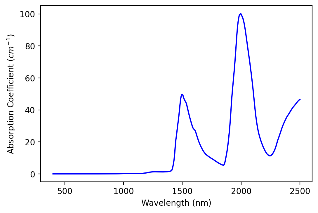
It’s hard to get an intuitive sense of the strength of absorption because of our units (cm-1). We can see that the values are higher in the SWIR than in the NIR and visible, indicating more absorption in these wavelengths. One way to make absorption strength more intuitive is to calculate e-folding distance spectra.
Calculate e-folding distance
We can calculate the e-folding distance to better visualize the absorption feature. This distance will occur when \(\alpha_\lambda d = 1\), so:
Solving for \(d\) gives us the equivalent thickness of a material needed to reproduce the absorption feature.
# Calculate e-folding distances in cm
ice_efld_fullres = 1 / ice_abs_fullres

# Plot e-folding distance
plt.plot(wvl_nm_fullres, ice_efld_fullres, color='blue')
plt.xlabel('Wavelength (nm)')
plt.ylabel('e-folding distance (cm)')
plt.xlim([900, 2500])
plt.ylim([0,8])
plt.show()
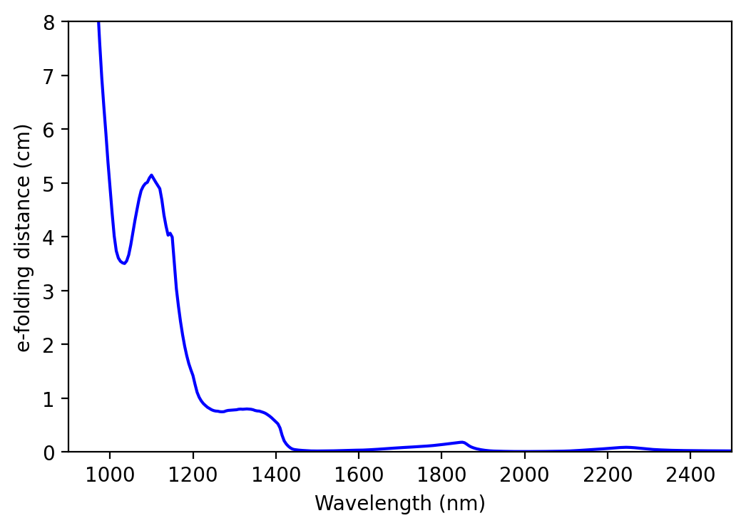
We can see that absorption is strong beyond 1400 nm. Thus, we will use the region of moderate absorption (between 900 and 1300 nm) for our spectral feature fitting (SFF).
Load the point of interest
Next, we will load a GeoJSON file that includes the point of interest, or the specific pixel in which we plan to explore.
roi = geopandas.read_file('https://raw.githubusercontent.com/snowex-hackweek/tutorial-data/main/SnowEx-2022/AVIRIS-NG/roi.geojson')
Start a new map
sasp = swamp_angel.explore(
    name='Swamp Angel Study Plot',
    tiles="Stamen Terrain"
)
Add our point of interest. Note that we need the coordinates in Lat/Lon to add it to our base map. Luckily, we can do that quickly with geopandas to_crs method.
See also
lat_lon = roi.to_crs(4326).geometry

folium.Marker(
    location=[lat_lon.y, lat_lon.x],
    icon=folium.Icon(color='orange'),
    popup='Point of Interest'
).add_to(sasp)

sasp
Find the coordinates in pixel space
import rasterio

with rasterio.open(SBB_data_file) as sbb_subset:
    x, y = sbb_subset.index(roi.geometry.x, roi.geometry.y) # The index methods returns arrays
    print(x[0], y[0])
31 54
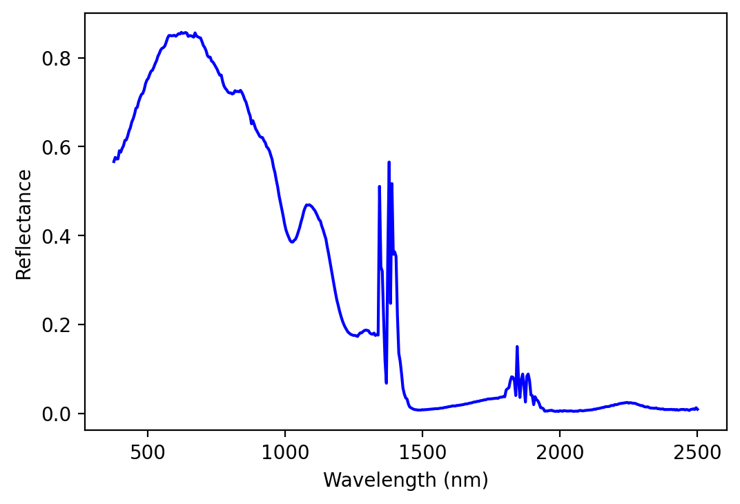
Show the measured reflectance at this pixel
#plot spectrum for a given pixel
my_pixel = image_data[x[0], y[0]]
plt.plot (bands, my_pixel, color='blue')
plt.xlabel('Wavelength (nm)')
plt.ylabel('Reflectance')
plt.show()
Align bands between image and reference spectra
To do spectral feature fitting, we need the bands in our water and ice absorption spectra to match the bands in our AVIRIS-NG image. Let’s use spline interpolation to convert our absorption spectra from 5 nm band centers to AVIRIS-NG band centers.
from scipy.interpolate import CubicSpline

# Create CubicSpline functions that use the original absorption spectra wavelengths and values
ice_cs = CubicSpline(wvl_nm_fullres, ice_abs_fullres)

# Interpolate to AVIRIS-NG band center wavelengths
ice_abs_imgres = ice_cs(bands)
Run Spectral Feature Fitting
Now that our absorption spectra have the same band center wavelengths as our image, we can move forward with the spectral feature fitting. The next step involves constraining the wavelength range we’ll be fitting. This can be a little tricky - a subjective choice about where absorption features begin and end needs to be made. Often, we’ll need to test multiple bounding wavelengths and choose a set that works best.
# Set the absorption feature wavelength bounds
lower_bound = 980
upper_bound = 1095

lower_bound_index = index_for_band(lower_bound)
upper_bound_index = index_for_band(upper_bound)
Next, we’ll want the wavelengths and bands to correspond to the range between these bounds.
# Remember: Numpy's upper bound index is excluded. Hence +1
bands_in_feature = bands[lower_bound_index:upper_bound_index + 1]
band_index_in_feature = np.arange(lower_bound_index, upper_bound_index + 1)
We can then use a nonnegative least squares approach to perform the spectral feature fitting, which has been noted as one of the most efficient methods (Thompson et al., 2015).
To do so, we need to solve for the following values:
\(l\): our offset
\(m\): slope of the upward-trending line
\(n\): slope of the downward-trending line
\(u_{ice}\): equivalent thickness of ice (called \(d_{ice}\) in our nonlinear solution)
Therefore we need to construct our x data array with the relevant vectors:
a vector of ones (will be used to find \(l\))
a vector of wavelengths (used to find \(m\))
a vector of wavelengths * -1 (used to find \(n\))
a vector of ice abs coefficients (used to find \(u_{ice}\))
We need our wavelengths and ice absorption coefficients in an array we can use as an input for SFF. The bands will be restricted to the bounds we’ve already defined. We’ll also want our reflectance spectrum in a similarly formatted array.
# Import 'nnls' and set up your x and y arrays
from scipy.optimize import nnls
x_values = np.transpose(
    np.array([
        np.ones_like(bands_in_feature),
        bands_in_feature,
        -1 * bands_in_feature,
        ice_abs_imgres[band_index_in_feature]
    ])
)
print(x_values.shape)

y_values = my_pixel[band_index_in_feature]
print(y_values.shape)
(24, 4)
(24,)
# Solve for a, b, and d_ice using nnls
coeff, resid = nnls(x_values, -np.log(y_values))
print(coeff)
[1.37507001e+00 0.00000000e+00 8.99078435e-04 1.77428070e+00]
# Look at the estimated ice thickness
print("estimated ice thickness = {}".format(round(coeff[3], 3)))
estimated ice thickness = 1.774
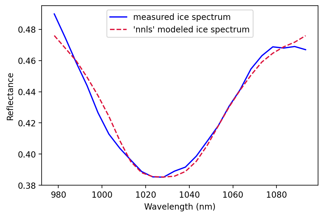
# Generate your modeled spectral feature
nnls_predicted_ice_abs = np.exp(-x_values.dot(coeff[:, np.newaxis]))
# Plot both over your measured spectral feature
plt.figure()
plt.plot(bands_in_feature, my_pixel[band_index_in_feature], color = 'blue')
plt.plot(bands_in_feature, nnls_predicted_ice_abs, color = 'crimson', linestyle = '--')
plt.legend(['measured ice spectrum',
            '\'nnls\' modeled ice spectrum'])
plt.xlabel('Wavelength (nm)')
plt.ylabel('Reflectance')
plt.show()
Wrapping it up
What we learned
Basic intro to hyperspectral data concepts
First intro working with AVIRIS-NG hyperspectral data and structure
Get overview of many flight lines, subset flight lines, and explore data for individual pixels
Used Python libraries:
Spectral (Read and explore hyperspectral data)
GeoPandas (Read and explore geospatail data)
Numpy (work with arrays)
Scipy (data science tools)
Matplotlib (static plots)
Folium (interactive maps)