.ipynb .pdf

repository open issue suggest edit

Binder

Contents

Introduction to Machine Learning

Compiled by: Ibrahim O. Alabi and Evi Ofekeze (Computing PhD, Data Science, Boise State University)

Learning Objectives

1. Understand the goals and main concepts of a Machine Learning Algorithm

2. Prepare a SnowEx dataset for Machine Learning

3. Understand the fundamental types of and techniques in Machine Learning

4. Implement Machine Learning with a SnowEx dataset

5. How to deploy a Machine Learning Model

What is Machine Learning?

Machine Learning simply means building algorithms or computer models using data. The goal is to use these “trained” computer models to make decisions.

Here is a general definition;

Machine Learning is the field of study that gives computers the ability to learn without being explicitly programmed (Arthur Samuel, 1959)

Over the years, ML algorithms have achieved great success in a wide variety of fields. Its success stories include disease diagnostics, image recognition, self-driving cars, spam detectors, and handwritten digit recognition. In this tutorial we will train a model using a SnowEx dataset.

Binary Example

Suppose we want to build a computer model that returns 1 if the input is a prime number and 0 otherwise. This model may be represented as follows;

\[Y = F(X)\]

Where:

• \(X \to\) the number entered also called a feature

• \(Y \to\) the outcome we want to predict

• \(F \to\) the model that gets the job done

Contrary to classical programming where we program the function, in Machine Learning we learn the function by training the algorithm with data.

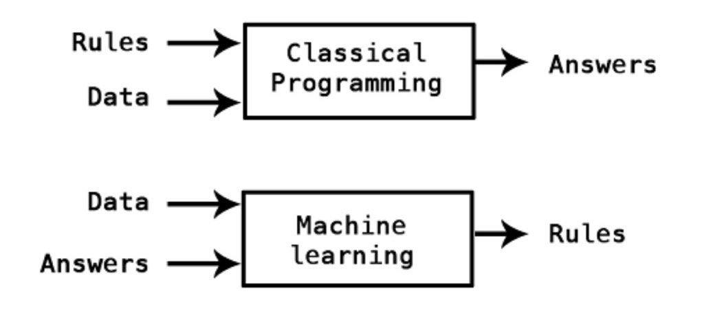
\(\qquad \qquad \qquad \qquad \qquad \qquad \qquad \qquad \qquad\) image by Kpaxs on Twitter

Machine Learning is useful when the function cannot be programmed or the relationship between the features and outcome is unknown.

SnowEx Data

Now we will import data from the 2017 SnowEx Airborne Campaign. In Machine Learning terminologies, it contains the following features;

• phase

• coherence

• amplitude

• incidence angle

and outcome

• snow depth

The goal is to use the data to learn the computer model \(F\) so that

snow depth = \(F\)(phase, coherence, amplitude, incidence angle)

Once \(F\) is learned, it can be used to predict snow depth given the features.

Load Dataset

Note that this dataset has been cleaned in a separate notebook, and it is available for anyone interested.

Load libraries:

import time
import numpy as np
import pandas as pd
import seaborn as sns
import matplotlib.pyplot as plt

from sklearn.preprocessing import MinMaxScaler
from sklearn.metrics import mean_squared_error, r2_score, mean_absolute_percentage_error, mean_absolute_error

dataset = pd.read_csv("./data/snow_depth_data.csv")
dataset.info()
dataset.head()

<class 'pandas.core.frame.DataFrame'>
RangeIndex: 3000 entries, 0 to 2999
Data columns (total 5 columns):
 #   Column      Non-Null Count  Dtype  
---  ------      --------------  -----  
 0   amplitude   3000 non-null   float64
 1   coherence   3000 non-null   float64
 2   phase       3000 non-null   float64
 3   inc_ang     3000 non-null   float64
 4   snow_depth  3000 non-null   float64
dtypes: float64(5)
memory usage: 117.3 KB

	amplitude	coherence	phase	inc_ang	snow_depth
0	0.198821	0.866390	-8.844648	0.797111	0.969895
1	0.198821	0.866390	-8.844648	0.797111	1.006760
2	0.212010	0.785662	-8.843649	0.799110	1.033615
3	0.212010	0.785662	-8.843649	0.799110	1.043625
4	0.173967	0.714862	-8.380865	0.792508	1.593430

Train and Test Sets

For the algorithm to learn the relationship pattern between the feature(s) and the outcome variable, it has to be exposed to examples. The dataset containing the examples for training a learning machine is called the train set (\(\mathcal{D}^{(tr)}\)).

On the other hand, the accuracy of an algorithm is measured on how well it predicts the outcome of observations it has not seen before. The dataset containing the observations not used in training the ML algorithm is called the test set (\(\mathcal{D}^{(te)}\)).

In practice, we divide our dataset into train and test sets, train the algorithm on the train set and evaluate its performance on the test set.

train_dataset = dataset.sample(frac=0.8, random_state=0)
test_dataset = dataset.drop(train_dataset.index)

Inspect the Data

Visualization

Before modelling, it is always a good idea to visualize our dataset. With visualization, we gain insights into the relationships between the variables and the shape of the distribution of each variable. For this data, we shall look into the scatterplot matrix.

sns.pairplot(train_dataset[['snow_depth','amplitude', 'coherence', 'phase', 'inc_ang']], diag_kind='kde');

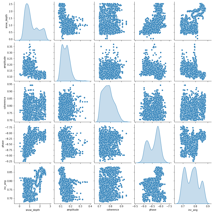
Each panel (excluding the main diagonal) of the scatterplot matrix is a scatterplot for a pair of variables whose identities are given by the corresponding row and column labels. The main diagonal is density plot for each variable. None of the features have a linear relationship with snow_depth. This may indicate that a linear model might not be the best option.

Descriptive Statistics

• count: the size of the training set

• mean: arithmetic mean

• std: sample standard deviation

• min: minimum value

• 25%: 25% of the values fall below this number

• 50%: 50\(^{th}\) percentile also called the median. 50% of the values fall below this number and 50% of the values fall above this number

• 75%: 75% of the values fall below this number

• max: maximum value

train_dataset.describe().transpose()

	count	mean	std	min	25%	50%	75%	max
amplitude	2400.0	0.151192	0.040073	0.077860	0.119580	0.148579	0.175531	0.368253
coherence	2400.0	0.778119	0.048796	0.700428	0.738597	0.773580	0.811030	0.942499
phase	2400.0	-8.419475	0.338714	-9.240785	-8.743792	-8.326929	-8.145543	-7.690262
inc_ang	2400.0	0.772514	0.054758	0.679981	0.719910	0.775250	0.809429	0.880183
snow_depth	2400.0	1.178734	0.629103	0.051438	0.667404	0.961838	1.652085	2.551194

Feature Engineering

Feature engineering means different things to different data scientists. However, in this tutorial, we will define feature engineering as the art of manipulating and transforming data into a format that optimally represents the underlying problem. In other words, any transformation/cleaning you do between data collection and model fitting may be called feature engineering.

Types of Feature Engineering

1. Feature improvement (normalization, missing value imputation, etc.).

2. Feature construction (creating new features from original data).

3. Feature selection (hypthesis testing, information gain from tree-based models).

4. Feature extraction (Principal Component Analysis (PCA), Singular Value Decomposition (SVD), etc.).

Normalization

The features and outcome are measured in different units and hence are on different scales. Machine Learning algorithms are very sensitive and important information can be lost if they are not on the same scale. A simple way to address this is to project all the variables onto the same scale, in a process known as Normalization.

Normalization simply consists of transforming the variables such that all values are in the unit interval [0, 1]. With Normalization, if \(X_j\) is one of the variables, and we have \(n\) observations \(X_{1j}, X_{2j}, \cdots, X_{nj}\), then the normalized version of \(X_{ij}\) is given by:

\[ \tilde{X}{ij} = \frac{X_{ij} - \min X_j}{\max X_j - \min X_j} \]

Note: whether the outcome variable should be normalized or not is an issue of preference. In this tutorial, we will not normalize the output variable. If you wish to normalize yours, you have to transform your predictions back to their original scales.

scaler = MinMaxScaler()
scaled_train_features = scaler.fit_transform(train_dataset.drop(columns=['snow_depth']))
scaled_test_features = scaler.transform(test_dataset.drop(columns=['snow_depth'])) ## fit_transform != transform. 
                                                                                   ## transform uses the parameters of fit_transform
                                                                                   ## DO NOT TRANSFORM YOUR TEST SET SEPARATELY, USE PARAMETERS LEARNED FROM TRAINING SET!!!!

Separate Features from Labels

Our last step for preparing the data for Machine Learning is to separate the features from the outcome.

train_X, train_y = scaled_train_features, train_dataset['snow_depth']
test_X, test_y = scaled_test_features, train_dataset['snow_depth']

Why Estimate \(F\)?

We estimate \(F\) for two main reasons;

1. Prediction: in this case, the features \(X\) are available, but there is no explicit rule for obtaining the outcome \(Y\).

2. Inference: in practice, we are sometimes interested in how changing the input \(X\) effects \(Y\). Inference can tell us which features are significantly associated with a particular outcome and the nature of the relationship between \(X\) and \(Y\).

How Do We Estimate \(F\)?

Machine Learning Algorithms

Machine learning algorithms can be categorized based on different criteria. In this tutorial, our categorization will be based on the amount and type of supervision needed during the training process. Based on this criterion, there are four major categories; supervised learning, unsupervised learning, semisupervised learning, and reinforcement learning. We shall limit our definition to the first two;

• Supervised Learning: this refers to tasks where we have a specific outcome to predict. That is, every observation of the features has a corresponding outcome. An example of a supervised learning task is predicting snow depth based on some influencing features.

• Unsupervised Learning: this refers to tasks where we have no outcome to predict. Here, rather than predict an outcome, we seek to understand the relationship between the features or between the observations or to detect anomalous observations. Considering the example above, we assume the snow depth variable does not exist and we either understand the relationship between the features or between the observations based on the features.

It is worth noting that a variable can either be categorical or continuous. For now, let’s focus on the nature of the outcome variable. In Supervised Learning parlance, if the outcome variable is categorical, we have a classification task and if continuous, we are in the presence of a regression task. Categorical implies that the variable is made of distinct categories (e.g. blood types: A, AB, O) and continuous implies that the variable is measured (e.g. snow depth). For the rest of this tutorial, we will focus on Supervised Learning tasks with a special concentration on regression tasks.

Machine Learning Installation Guide

For this notebook to run successfully, you have to install the following packages;

1. TensorFlow

2. Keras

Tensorflow: it is an end-to-end open source platform for machine learning. It makes it easy to train and deploy machine learning models. TensorFlow was created at Google and supports many of their large-scale Machine Learning applications. Read more at About TensorFlow.

Keras: Keras is a deep learning Application Programming Interface (API) written in Python, running on top of the machine learning platform TensorFlow. It was developed with a focus on enabling fast experimentation. Read more at About Keras.

Other packages needed come pre-installed in Anaconda.

You only need to install TensorFlow as Keras comes as a submodule in TensorFlow. To install TensorFlow, launch the Jupyter Lab Terminal and type the following command:

       \(\texttt{C:\Users\Default> pip install tensorflow}\)

After installation, you will be able to continue with the tutorial. For this tutorial, both Tensorflow and Keras used are version 2.8

Most Machine Learning techniques can be characterised as either parametric or non-parametric.

Parametric: The parametric approach simplifies the problem of estimating \(F\) to a parameter estimation problem. The disadvantage is that we assume a particular shape of \(F\) that may not match the true shape of \(F\). The major advantage of using parametric approach that when inference is the goal we can understand how changing \(X_1, X_2, \cdots, X_k\) effects \(Y\). A common parametric method is the Linear Regression.

Non-parametric: Non-parametric approaches do not assume any shape for \(F\). Instead, they try to estimate \(F\) that gets as close to the data points as possible. The disadvantage of non-parametric approaches is that they require extensive training observations to estimate \(F\) accurately. Common examples of non-parametric methods include Random Forest, Neural Networks, and support vector machines.

In this tutorial, we will focus on non-parametric approaches with a specific concentration on Random Forest and Neural networks.

Random Forest

Random forest is a simple but powerful algorithm that handles classification and regression tasks. The structural building blocks of Random Forest are decision trees; we will begin our explanation with decision trees. When we use decision trees for regression tasks, we call them regression trees; when we use decision trees for classification tasks, we call them classification trees. Subsequently, we use “regression trees” instead of “decision trees” because we will solve a regression problem in this tutorial.

Regression Trees

Consider a dataset \(\mathcal{D}_n = \left\lbrace (\textbf{x}_1, y_1), (\textbf{x}_2, y_2), \cdots, (\textbf{x}_n, y_n) \right\rbrace\) where \(\textbf{x}_i^\top \equiv ({x}_{i1}, {x}_{i2}, \cdots, {x}_{ik})\) denotes the \(k\)-dimensional vector of features, and \(y_i\) represents the corresponding outcome (continuous in this case).

The fundamental concept underlying regression trees is to split the feature space (set of possible values for the features) into two sub-regions. The sub-regions are further divided into two until a stopping criterion is reached. The predicted value of a given observation is the arithmetic mean of the training observations in the region it belongs.

Performance Evaluation

Each time we estimate the true outcome (\(Y\)) using a trained ML algorithm (\(F(X)\)), the discrepancy between the observed and predicted must be quantified. The question is, how do we quantify this discrepancy? This brings the notion of loss function.

Loss Function \(\mathcal{L} (\cdot,\cdot)\) is a bivariate function that quantifies the loss (error) we sustain from predicting \(Y\) with \(F(X)\). Put another way, loss function quantifies how close the prediction \(F(X)\) is to the ground truth \(Y\).

• Regression Loss Function

There exists quite a number of ways for which the loss of a regression problem may be quantified. We now illustrate two of them;

\[ \mathcal{L} (Y,F(X)) = (Y - F(X))^2 \]

This is popularly known as the squared error loss and it is simply the square of the difference between the observed and the predicted values. The loss is squared so that the function reaches its minimum (convex).

\[ \mathcal{L} (Y,F(X)) = |Y - F(X)| \]

Another way to quantify regression loss is by taking the absolute value of the difference between the observed (\(Y\)) and the predicted (\(F(X)\)) values. This is called the L1 loss.

It is worth noting that the loss function as defined above corresponds to a single observation. However, in practice, we want to quantify the loss over the entire dataset and this is where the notion of empirical risk comes in. Loss quantified over the entire dataset is called the empirical risk. Our goal in ML is to develop an algorithm such that the empirical risk is as minimum as possible. Empirical risk is also called the cost function or the objective function we want to minimize.

• Regression Empirical Risk

\[ \widehat{\mathcal{R}}_n(F) = \frac{1}{n}\sum_{i=1}^n{\mathcal{L}(Y_i, F(X_i))} \]

The empirical risk corresponding to the squared error loss is called “mean squared error”, while the empirical risk corresponding to the L1 loss is called “mean absolute error”. Other Regression Loss functions can be found at Keras: losses

Random Forest Setup

Load Random forest Libraries:

from sklearn.pipeline import Pipeline
from sklearn.ensemble import RandomForestRegressor
from sklearn.tree import DecisionTreeRegressor, plot_tree
from sklearn.model_selection import train_test_split, GridSearchCV

Regression Tree

The sklearn documentation for regression tree can be found here.

tree = DecisionTreeRegressor(random_state=0, max_depth=2)  ## random_state=0 for reproducible results
tree.fit(train_dataset.drop(columns='snow_depth'), 
         train_dataset['snow_depth'])

DecisionTreeRegressor(max_depth=2, random_state=0)

In a Jupyter environment, please rerun this cell to show the HTML representation or trust the notebook.
On GitHub, the HTML representation is unable to render, please try loading this page with nbviewer.org.

features = list(train_dataset.columns[:-1])

plt.figure(figsize = (20, 8))
plot_tree(tree, 
          filled = True, 
          fontsize = 12,
          node_ids = True,
          rounded = True,
          proportion=True,
         feature_names= features)
plt.show()

Now let’s explain the regression tree above

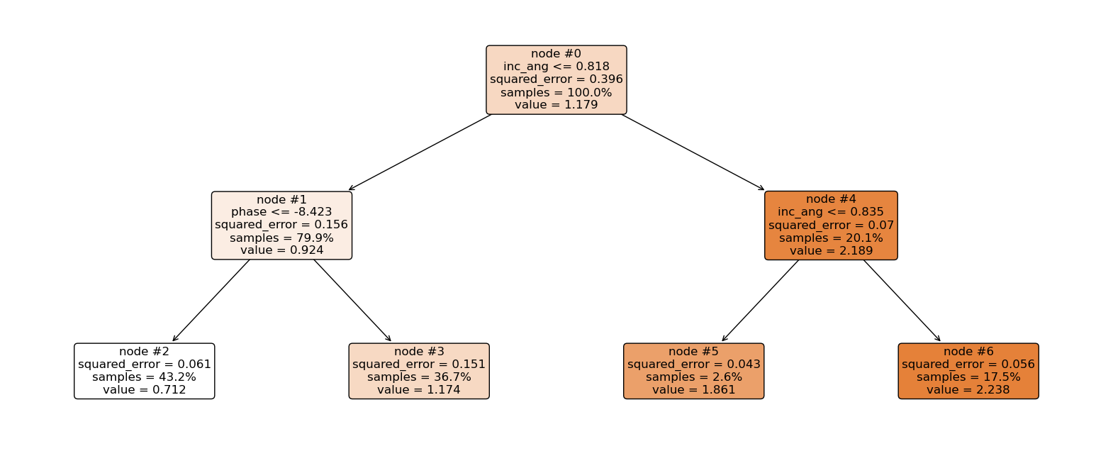
The root node (node #0) assigns values of incidence angle lesser than or equal to 0.818 to the right branch and values of incidence angle greater than 0.818 to the left node. Observations with incidence angle lesser than or equal to 0.818 are further partitioned based on phase values. Overall, the regression tree splits the observations into four disjoint groups or regions (\(R_i\)) of the feature space.

\begin{align*} R_1 &= \left\lbrace X \ | \ \text{inc_angle} \le 0.818,\ \text{phase} \le -8.423 \right\rbrace \qquad \quad \hat{y}{R_1} = 0.712 \ R_2 &= \left\lbrace X \ | \ \text{inc_angle} \le 0.818,\ \text{phase} > -8.423 \right\rbrace \qquad \quad \hat{y}{R_2} = 1.174 \ R_3 &= \left\lbrace X \ | \ \text{inc_angle} > 0.818,\ \text{inc_angle} \le 0.835 \right\rbrace \qquad \hat{y}{R_3} = 1.861 \ R_4 &= \left\lbrace X \ | \ \text{inc_angle} > 0.818,\ \text{inc_angle} > 0.835 \right\rbrace \qquad \hat{y}{R_4} = 2.238 \ \end{align*}

where \(\hat{y}_{R_i}\) is the mean of the respective regions. The regions \(R_i, \ i = 1,2,3, 4\) are called terminal nodes or leaves, the points where the feature space (\(X\)) is partitioned are called internal nodes and the line segments connecting the nodes are referred to as branches. Generally, to know which region an observation belongs to, we ask series of question(s) starting from the root node until we get to the terminal node and the value predicted for the observation is mean of all training observations in that region. Mathematically we write; \begin{equation} \hat{y} = \hat{f}(\text{x}) = \frac{1}{|R_j|} \sum_{i = 1}^{n} y_i 1(\text{x}_i \in R_j). \end{equation}

Here, if the \(i\)th observation belongs to region \(R_j\), the indicator function equals 1, else, it equals zero.

• Root node: node #0.

• Internal nodes: node #1 and node #4.

• Terminal nodes: node #2, node #3, node #5, and node #6.

We have mentioned the recursive splitting of observations into regions, the natural question that comes to mind is, how do we construct the regions? Our goal is to find regions such that the expected loss is minimized. To perform the recursive binary splitting, we consider all features in the feature space and all possible cut-point(s) for the individual features. The feature and cut-point leading to the greatest reduction in expected loss are chosen for splitting. This process is then continued until a stopping criterion is reached. A stopping criterion could be until no region contains more than five observations. In sklearn, the stopping criterion is controlled by \(\texttt{max_depth}\) and \(\texttt{min_samples_split}\).

How to make predictions

An example:

sample = test_dataset.loc[[0], ['amplitude', 'coherence', 'phase', 'inc_ang']]
sample

	amplitude	coherence	phase	inc_ang
0	0.198821	0.86639	-8.844648	0.797111

tree.predict(sample)

array([0.71192304])

• incidence angle is lesser than 0.818 and phase is lesser than -8.423. This falls in region one (\(R_1\)), and our prediction will be 0.712.

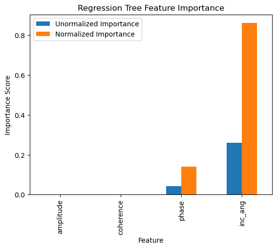
Feature Importance

The total amount by which the empirical risk is decreased due to splits over a given predictor is documented. The larger the value, the more important the variable. Sklearn’s implementation of variable importance normalizes the variable importance so that they add up to 1. Mathematically, feature importance is computed as:

\[I_j= \sum_j w_jC_j - w_{left(j)}C_{left(j)} - w_{right(j)}C_{right(j)}\]

• \(I_j\)= importance of variable \(j\)

• \(C_j\)= the MSE of node \(j\)

• \(w_j\)= percentage of the observation reaching node \(j\)

## compute inc_ang importance

node0=0.396 - 0.799*0.156 - 0.201*0.07
node4=0.201*0.07 - 0.026*0.043 - 0.175*0.056
imp_inc_ang=node0+node4

## compute phase importance

imp_phase=0.799*0.156 - 0.432*0.061 - 0.151*0.367 
print('Incidence Angle Importance: {}, Phase Importance: {}'.format(imp_inc_ang,imp_phase))

Incidence Angle Importance: 0.260438, Phase Importance: 0.04287500000000001

feature_impotanceRT = pd.DataFrame({
    'Unormalized Importance': tree.tree_.compute_feature_importances(normalize=False),
    'Normalized Importance': tree.feature_importances_
}, index=features)
feature_impotanceRT

	Unormalized Importance	Normalized Importance
amplitude	0.000000	0.000000
coherence	0.000000	0.000000
phase	0.042388	0.139957
inc_ang	0.260475	0.860043

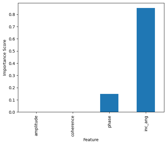
feature_impotanceRT.plot(kind = 'bar')
plt.title('Regression Tree Feature Importance')
plt.xlabel('Feature')
plt.ylabel('Importance Score')
plt.show()

Exercise:

Compute the normalized importance manually and compare it with sklearn’s output above.

Random Forest

If you want to go fast, go alone. If you want to go far, go together (African Proverb).

Regression trees suffer from high variance, that is, they have a habit of overfitting the training observations. A straightforward way to reduce the variance is to employ the Random Forest (RF) algorithm. RF is an ensemble learning technique that can be used for both classification and regression. The term “ensemble learning” means combining multiple algorithms to obtain an improved version of the constituting algorithms. RF does this using the concept of Bagging.

• Bagging: Bagging consists of two words; Bootstrap and Aggregation. Bootstrap is a popular resampling technique where random sub-samples (with replacement) are created from the training data. The individual bootstrapped sub-sample is called a “Bag.” Aggregation, however, means combining the results from machines trained on the respective bags. We could say, given our training data, we generate \(B\) bootstrapped training sub-samples from the original training data, then we train an algorithm on the respective bootstrapped sub-sample to obtain \(\hat{F}^1 (\text{x}), \hat{F}^2 (\text{x}), \cdots , \hat{F}^B (\text{x})\). The final predicted value is the average of all the individual predictions and it is given by: \begin{equation} \hat{F}{\text{bag}} (\text{x}) = \frac{1}{B} \sum{b = 1}^{B} \hat{F}^{b} (\text{x}). \end{equation}

This is bagging! In the RF algorithm, regression trees are built on the different bootstrapped samples and the result is a forest of regression trees, hence the “forest” in Random Forest.

• What makes the forest random?

Recall that when training a regression tree, splitting is done at each internal node, however, in the RF algorithm, when building the individual regression trees, only a random sample of the total features is considered for optimal splitting and this is what makes the forest random! In essence, when we combine bagging with random feature selection at each internal node of the constituting regression trees, we are said to have constructed a Random Forest learning machine.

Training Random Forest

Sklearn’s documentation for Random Forest Regression can be found here. The documentation can also be gotten directly from your Jupyter Notebook using the help function as shown below.

#help(RandomForestRegressor)

rf = RandomForestRegressor(n_estimators=2,max_depth=2,random_state=0)

rf.fit(train_dataset.drop(columns='snow_depth'), 
         train_dataset['snow_depth'])

RandomForestRegressor(max_depth=2, n_estimators=2, random_state=0)

In a Jupyter environment, please rerun this cell to show the HTML representation or trust the notebook.
On GitHub, the HTML representation is unable to render, please try loading this page with nbviewer.org.

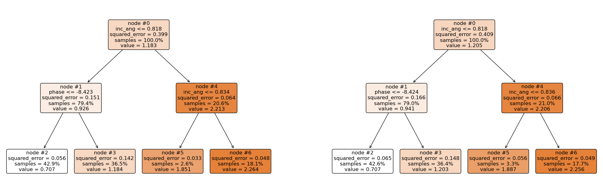
plt.figure(figsize = (25, 8))

plt.subplot(121)
plot_tree(rf.estimators_[0], 
          filled = True, 
          fontsize = 12,
          node_ids = True,
          rounded = True,
          proportion=True, 
         feature_names= features)

plt.subplot(122)
plot_tree(rf.estimators_[1], 
          filled = True, 
          fontsize = 12,
          node_ids = True,
          rounded = True,
          proportion=True, 
         feature_names= features)

plt.show()

Making Predictions

sample

	amplitude	coherence	phase	inc_ang
0	0.198821	0.86639	-8.844648	0.797111

## Overall predictions

rf.predict(sample)

array([0.70685414])

## Prediction from the first tree

rf.estimators_[0].predict(sample)

/usr/share/miniconda3/envs/hackweek/lib/python3.10/site-packages/sklearn/base.py:443: UserWarning: X has feature names, but DecisionTreeRegressor was fitted without feature names
  warnings.warn(

array([0.70719868])

## Prediction from the second tree

rf.estimators_[1].predict(sample)

/usr/share/miniconda3/envs/hackweek/lib/python3.10/site-packages/sklearn/base.py:443: UserWarning: X has feature names, but DecisionTreeRegressor was fitted without feature names
  warnings.warn(

array([0.7065096])

Using the same approach as above, the first regression tree predicts 0.7072, and the second regression tree predicts 0.7065. Hence, the final prediction is;

\[\frac{0.7072+0.7065}{2} = 0.70685\]

Feature Importance

The total amount by which the squared error loss is decreased due to splits over a given predictor is documented and averaged over all trees in the forest. The larger the value, the more important the variable.

feature_impotanceRF = pd.Series(rf.feature_importances_, index=features)
feature_impotanceRF.plot(kind = 'bar')
plt.xlabel('Feature')
plt.ylabel('Importance Score')
plt.show()

Exercise:

Compute the random forest’s normalized importance manually and compare it with sklearn’s output above.

Putting it all together

We’ll use Sklearn’s Pipeline to preprocess and fit our model in one shot.

rf_pipe = Pipeline([
    ('Scaler', MinMaxScaler()),
    ('regressor', RandomForestRegressor())
])

rf_pipe.fit(train_dataset.drop(columns='snow_depth'), 
         train_dataset['snow_depth'])

Pipeline(steps=[('Scaler', MinMaxScaler()),
                ('regressor', RandomForestRegressor())])

In a Jupyter environment, please rerun this cell to show the HTML representation or trust the notebook.
On GitHub, the HTML representation is unable to render, please try loading this page with nbviewer.org.

Neural Networks

Neural networks are learning machines inspired by the functionality of biological neurons. They are not models of the brain, because there is no proven evidence that the brain operates the same way neural networks learn representations. However, some of the concepts were inspired by understanding the brain. Every NN consists of three distinct layers;

1. Input layer

2. Hidden layer(s) and

3. Output layer.

To understand the functioning of these layers, we begin by exploring the building blocks of neural networks; a single neuron or perceptron.

A perceptron or Single Neuron

Each layer in a NN consists of small individual units called neurons (usually represented with a circle). A neuron receives inputs from other neurons, performs some mathematical operations, and then produces an output. Each neuron in the input layer represents a feature. In essence, the number of neurons in the input layer equals the number of features. Each neuron in the input layer is connected to every neuron in the hidden layer. The number of neurons in the hidden layer is not fixed, it is problem dependent and it is often determined via cross-validation or validation set approach in practice.

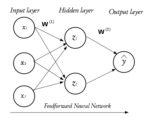
The configuration of the hidden layer(s) controls the complexity of the network. A NN may contain more than one hidden layer. A NN with more than one hidden layer is called a deep neural network while that with a single hidden layer is a shallow neural network. The final layer of a neural network is called the output layer and it holds the predicted outcomes of observations passed into the input layer. Every inter-neuron connection has an associated weight, these weights are what the neural network learns during the training process. When connections between the layers do not form a loop, such networks are called feedforward neural networks and if otherwise, they are called recurrent neural networks. In this tutorial, we shall concentrate on the feed forward neural networks.

How the perceptron works

Consider a dataset \(\mathcal{D}_n = \left\lbrace (\textbf{x}_1, y_1), (\textbf{x}_2, y_2), \cdots, (\textbf{x}_n, y_n) \right\rbrace\) where \(\textbf{x}_i^\top \equiv ({x}_{i1}, {x}_{i2}, \cdots, {x}_{ik})\) denotes the \(k\)-dimensional vector of features, and \(y_i\) represents the corresponding outcome. Given a set of input fed into the network through the input layer, the output of a neuron in the hidden layer is

\[ f(\textbf{x}_i;\textbf{w}) = g(w_0 + \textbf{w}^\top \textbf{x}_i), \]

where \(\textbf{w} = (w_1, w_2, \cdots, w_k)^\top\) is a vector of weights and \(w_0\) is the bias term associated with the neuron. The weights can be thought of as the slopes in a linear regression and the bias as the intercept. The function \(g(\cdot)\) is known as the activation function and it is used to introduce non-linearity into the network.

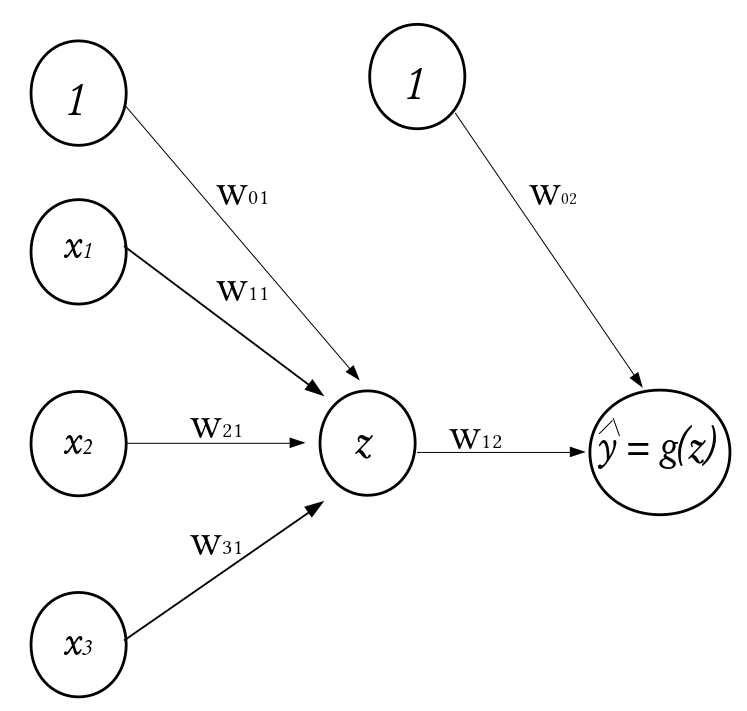
\(\qquad \qquad \qquad \qquad \qquad \qquad \qquad \qquad \qquad \qquad \qquad\) A Perceptron

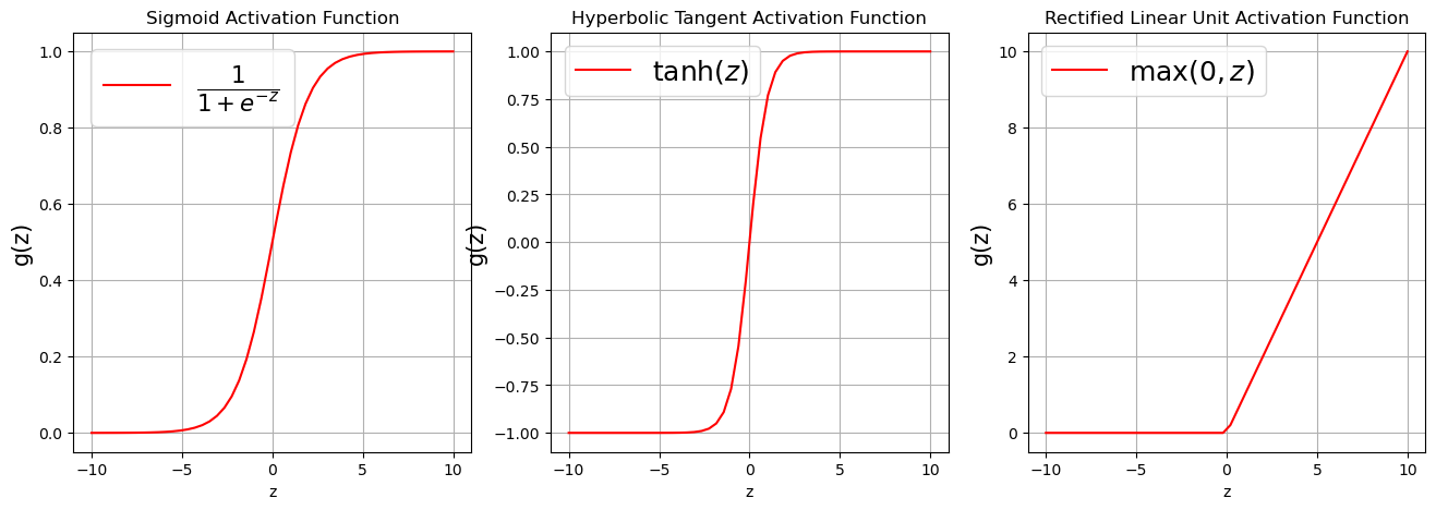
There exists a number of activation functions in practice, the commonly used ones are

1. Sigmoid or Logistic activation function $\(g(z) = \frac{1}{1 + e^{-z}}.\)$

2. Hyperbolic Tangent activation function $\(g(z) = \tanh (z) = \frac{e^{z}-e^{-z}}{e^{z}+e^{-z}}.\)$

3. Rectified Linear Unit activation function $\(g(z) = \max(0,z).\)$

Visualizing Activation Functions

def Sigmoid(z):
    """
    A function that performs the sigmoid transformation
    
    Arguments:
    ---------
        -* z: array/list of numbers to activate
    
    Returns:
    --------
        -* logistic: the transformed/activated version of the array
    """
    
    logistic = 1/(1+ np.exp(-z))
    return logistic
    

def Tanh(z):
    """
    A function that performs the hyperbolic tangent transformation
    
    Arguments:
    ---------
        -* z: array/list of numbers to activate
    
    Returns:
    --------
        -* hyp: the transformed/activated version of the array
    """
    
    hyp = np.tanh(z)
    return hyp


def ReLu(z):
    """
    A function that performs the hyperbolic tangent transformation
    
    Arguments:
    ---------
        -* z: array/list of numbers to activate
    
    Returns:
    --------
        -* points: the transformed/activated version of the array
    """
    
    points = np.where(z < 0, 0, z)
    return points

z = np.linspace(-10,10)
fa = plt.figure(figsize=(16,5))

plt.subplot(1,3,1)
plt.plot(z,Sigmoid(z),color="red", label=r'$\frac{1}{1 + e^{-z}}$')
plt.grid(True, which='both')
plt.xlabel('z')
plt.ylabel('g(z)', fontsize=15)
plt.title("Sigmoid Activation Function")
plt.legend(loc='best',fontsize = 22)


plt.subplot(1,3,2)
plt.plot(z,Tanh(z),color="red", label=r'$\tanh (z)$')
plt.grid(True, which='both')
plt.xlabel('z')
plt.ylabel('g(z)', fontsize=15)
plt.title("Hyperbolic Tangent Activation Function")
plt.legend(loc='best',fontsize = 18)

plt.subplot(1,3,3)
plt.plot(z,ReLu(z),color="red", label=r'$\max(0,z)$')
plt.grid(True, which='both')
plt.xlabel('z')
plt.ylabel('g(z)', fontsize=15)
plt.title("Rectified Linear Unit Activation Function")
plt.legend(loc='best', fontsize = 18)

<matplotlib.legend.Legend at 0x7f507df1f310>

Families of Neural Networks

1. Feedforward Neural Networks: often used for structured data.

2. Convolutional Neural Networks: the gold standard for computer vision.

3. Transfer Learning: reusing knowledge from previous tasks on new tasks.

4. Recurrent Neural Networks: well suited for sequence data such as texts, time series, drawing generation.

5. Encoder-Decoders: commonly used for but not limited to machine translation.

6. Generative Adversarial Networks: usually used for 3D modelling for video games, animation, etc.

7. Graph Neural Networks: usually used to work with graph data.

Neural Network Setup

Load libraries:

import tensorflow as tf # Keras is part of standard TensorFlow library (Keras is available as a submodule in the TensorFlow library)

### Check the version of Tensorflow and Keras
print("TensorFlow version ==>", tf.__version__) 
print("Keras version ==>",tf.keras.__version__)

TensorFlow version ==> 2.8.0
Keras version ==> 2.8.0

Feedforward Neural Network

• Specify Architecture

Here, we shall include three hidden layers with 1000, 512, and 256 neurons respectively. Layers added using the “\(\texttt{network.add(\)\cdots\()}\)” command.

tf.random.set_seed(1000)  ## For reproducible results
network = tf.keras.models.Sequential() # Specify layers in their sequential order
# inputs are 4 dimensions (4 dimensions = 4 features)
# Dense = Fully Connected.   
# First hidden layer has 1000 neurons with relu activations.
# Second hidden layer has 512 neurons with relu activations
# Third hidden layer has 256 neurons with Sigmoid activations
network.add(tf.keras.layers.Dense(1000, activation='relu' ,input_shape=(train_X.shape[1],)))
network.add(tf.keras.layers.Dense(512, activation='relu')) # sigmoid, tanh
network.add(tf.keras.layers.Dense(256, activation='sigmoid'))
# Output layer uses no activation with 1 output neurons
network.add(tf.keras.layers.Dense(1)) # Output layer

2024-03-01 22:52:27.564374: I tensorflow/core/platform/cpu_feature_guard.cc:151] This TensorFlow binary is optimized with oneAPI Deep Neural Network Library (oneDNN) to use the following CPU instructions in performance-critical operations:  SSE4.1 SSE4.2 AVX AVX2 FMA
To enable them in other operations, rebuild TensorFlow with the appropriate compiler flags.

• Compile

The learning rate controls how the weights and bias are optimized. A discussion of the optimization procedure for Neural Networks can be found in Appendix B. If the learning rate is too small the training may get stuck, while if it is too big the trained model may be unreliable.

opt = tf.keras.optimizers.Adam(learning_rate=0.0001)
network.compile(optimizer = opt, loss='mean_squared_error', 
                metrics = [tf.keras.metrics.RootMeanSquaredError()])

• Print Architecture

network.summary()

Model: "sequential"

_________________________________________________________________

 Layer (type)                Output Shape              Param #   

=================================================================

 dense (Dense)               (None, 1000)              5000      

 dense_1 (Dense)             (None, 512)               512512    

 dense_2 (Dense)             (None, 256)               131328    

 dense_3 (Dense)             (None, 1)                 257       

=================================================================

Total params: 649,097

Trainable params: 649,097

Non-trainable params: 0

_________________________________________________________________

Number of weights connecting the input and the first hidden layer = (1000 \(\times\) 4) + 1000(bias) = 5000

• 4 = \(\texttt{number of features}\)

• 1000 = \(\texttt{number of nodes in the first hidden layer}\)

Number of weights connecting the first hidden layer and the second hidden layer = (1000 \(\times\) 512) + 512(bias) = 512512

• 512 = \(\texttt{number of nodes in the second hidden layer}\)

• 1000 = \(\texttt{number of nodes in the first hidden layer}\)

Number of weights connecting the second hidden layer and the third hidden layer = (512 \(\times\) 256) + 256(bias) = 131328

• 256 = \(\texttt{number of nodes in the third hidden layer}\)

• 512 = \(\texttt{number of nodes in the second hidden layer}\)

Number of weights connecting the third (last) hidden and the output layers = (256 \(\times\) 1) + 1(bias) = 257

• 256 = \(\texttt{number of nodes in the third hidden layer}\)

• 1 = \(\texttt{number of nodes in the output layer}\)

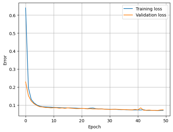
• Fit Model

Here we find the neural network weights using the data in the training set. An epoch is when an entire batch of the training set has been used. The number of times we iterate over the dataset is known as the number of epochs. The validation split is the fraction of the training set that will be used to evaluate the loss at the end of each epoch.

start_time = time.time()
# NOTE: Change to verbose=1 for per-epoch output
history =network.fit(train_X, train_y, epochs=50, validation_split = 0.2, verbose=0)
print('Total time taken (mins): ', round(float((time.time()-start_time)/60),2))

Total time taken (mins):  0.16

plt.plot(history.history['loss'], label='Training loss')
plt.plot(history.history['val_loss'], label='Validation loss')
plt.xlabel('Epoch')
plt.ylabel('Error')
plt.legend()
plt.grid(True)

Prediction

We have used Machine Learning to build two computer models \(F\) with SnowEx data. Now we will use the computer models to estimate snow depth for a given set of features (phase, coherence, amplitude, incidence angle).

## Random Forest

yhat_RF = rf_pipe.predict(test_dataset.drop(columns=['snow_depth']))


## Feed Forward Neural Network
yhat_dnn = network.predict(test_X).flatten() 


## True Snow Depth (Test Set)
observed = test_dataset["snow_depth"].values


## Put Observed and Predicted (Linear Regression and DNN) in a Dataframe
prediction_df = pd.DataFrame({"Observed": observed,
                    "RF":yhat_RF, "DNN":yhat_dnn})

Check Performance

def evaluate_model(y_true, y_pred, model_name, dp = 2):
    RMSE = np.sqrt(mean_squared_error(y_true=y_true, y_pred=y_pred)).round(dp)
    MAE  = mean_absolute_error(y_true=y_true, y_pred=y_pred).round(dp)
    MAPE = mean_absolute_percentage_error(y_true=y_true, y_pred=y_pred).round(dp)*100
    RSQ  = r2_score(y_true=y_true, y_pred=y_pred).round(dp)*100
    
    score_df = pd.DataFrame({
        model_name: [RMSE, MAE, MAPE, RSQ]
    }, index = ['RMSE(in)', 'MAE(in)', 'MAPE(%)', 'RSQ(%)'])
    
    return score_df

RF_evaluation=evaluate_model(prediction_df.RF, prediction_df.Observed, 'Random Forest')
NN_evaluation=evaluate_model(prediction_df.DNN, prediction_df.Observed, 'Neural Network')

comparison=pd.concat([RF_evaluation, NN_evaluation], axis=1)
comparison

	Random Forest	Neural Network
RMSE(in)	0.18	0.30
MAE(in)	0.11	0.22
MAPE(%)	11.00	20.00
RSQ(%)	92.00	76.00

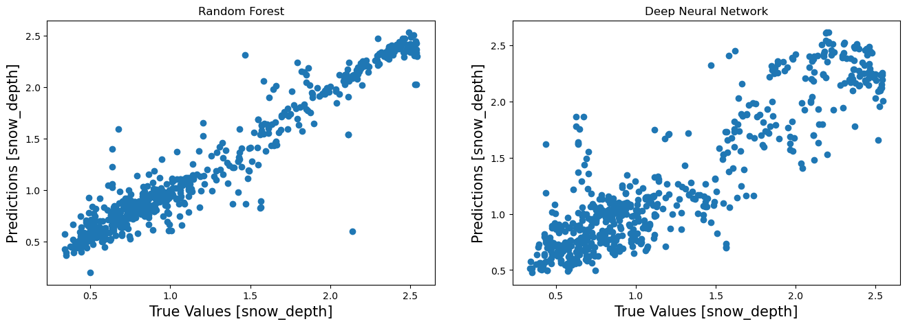
Visualize Performance

fa = plt.figure(figsize=(16,5))
plt.subplot(1,2,1)
plt.scatter(prediction_df['Observed'],prediction_df['RF'])
plt.xlabel('True Values [snow_depth]', fontsize=15)
plt.ylabel('Predictions [snow_depth]', fontsize=15)
plt.title("Random Forest")


plt.subplot(1,2,2)
plt.scatter(prediction_df['Observed'],prediction_df['DNN'])
plt.xlabel('True Values [snow_depth]', fontsize=15)
plt.ylabel('Predictions [snow_depth]', fontsize=15)
plt.title("Deep Neural Network")

Text(0.5, 1.0, 'Deep Neural Network')

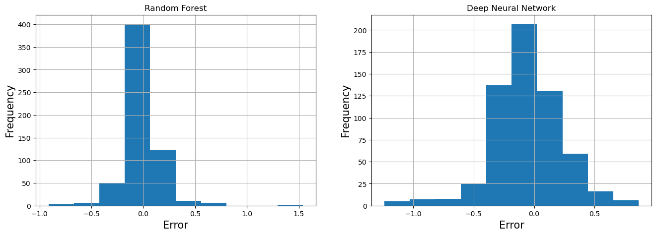
Visualize Error

RF_error = prediction_df['Observed'] - prediction_df['RF']
DNN_error = prediction_df['Observed'] - prediction_df['DNN']

fa = plt.figure(figsize=(16,5))

plt.subplot(1,2,1)
RF_error.hist()
plt.xlabel('Error', fontsize=15)
plt.ylabel('Frequency', fontsize=15)
plt.title("Random Forest")

plt.subplot(1,2,2)
DNN_error.hist()
plt.xlabel('Error', fontsize=15)
plt.ylabel('Frequency', fontsize=15)
plt.title("Deep Neural Network")

plt.show()

Main Challenges of Machine Learning

1. Bad Data (insufficient training data, nonrepresentative training data, irrelevant features)

2. Bad Algorithm (overfitting the training the data, underfitting the training data)

Improving your Model

Here are some ways to improve your machine learning models;

1. Regularization (early stopping, dropout, etc)

2. Hyperparameter Optimization

Hyperparameter Optimization

Hyperameters are parameters that are a step above other model parameters because their values have to be specified before fitting the model. They are not learned during the training process. In practice, different values are often “tuned” to obtain the optimal value, called hyperparameter optimization. Hyperparameter optimization is often done via a cross-validation (CV) or validation set approach.

• In the validation set approach, we hold out a portion of the training set and use the held-out portion to test the performance of different hyperparameters.

• Cross-validation: the training data is divided into k disjoint sets. The idea is to use one of the k folds as test set and the remaining k − 1 folds as training set. The algorithm then changes the test set until every fold has served as test set. Performance metric is computed at each iteration and averaged in the end.Sklearn’s implementation of grid search cross validation can be found here.

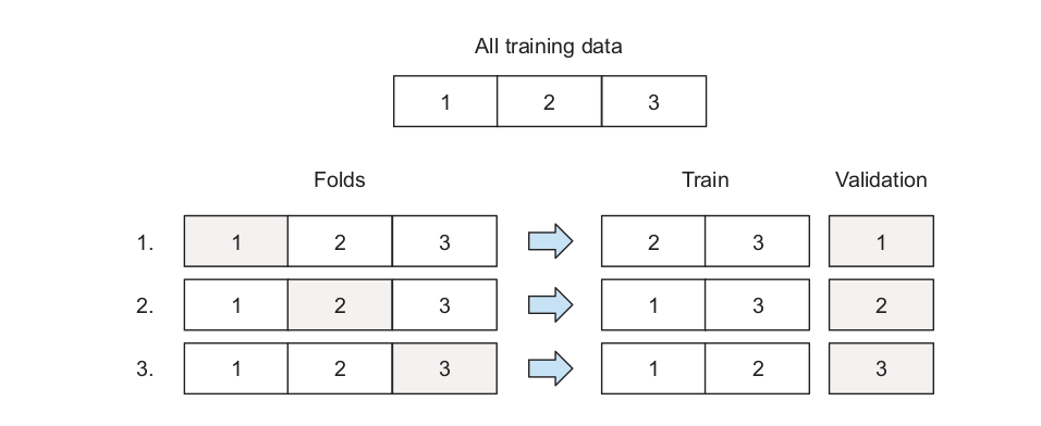
\(\qquad \qquad \qquad \qquad\) Source Machine Learning Bookcamp

• Random Forest Cross-validation

rf_pipe.get_params() #list of hyperparameters you may tune

{'memory': None,
 'steps': [('Scaler', MinMaxScaler()), ('regressor', RandomForestRegressor())],
 'verbose': False,
 'Scaler': MinMaxScaler(),
 'regressor': RandomForestRegressor(),
 'Scaler__clip': False,
 'Scaler__copy': True,
 'Scaler__feature_range': (0, 1),
 'regressor__bootstrap': True,
 'regressor__ccp_alpha': 0.0,
 'regressor__criterion': 'squared_error',
 'regressor__max_depth': None,
 'regressor__max_features': 1.0,
 'regressor__max_leaf_nodes': None,
 'regressor__max_samples': None,
 'regressor__min_impurity_decrease': 0.0,
 'regressor__min_samples_leaf': 1,
 'regressor__min_samples_split': 2,
 'regressor__min_weight_fraction_leaf': 0.0,
 'regressor__n_estimators': 100,
 'regressor__n_jobs': None,
 'regressor__oob_score': False,
 'regressor__random_state': None,
 'regressor__verbose': 0,
 'regressor__warm_start': False}

from sklearn.model_selection import GridSearchCV

parameter_grid = {'regressor__min_samples_split': [2,3],
                  'regressor__n_estimators': [50, 100], 
                  'regressor__max_depth': [3, 5]}

rf_pipeline_CV = GridSearchCV(rf_pipe, parameter_grid, verbose=1, cv=3) ## set njobs = -1 to use all processors. cv defaults to 5
rf_pipeline_CV.fit(train_dataset.drop(columns=['snow_depth']), 
         train_dataset['snow_depth'])

Fitting 3 folds for each of 8 candidates, totalling 24 fits

GridSearchCV(cv=3,
             estimator=Pipeline(steps=[('Scaler', MinMaxScaler()),
                                       ('regressor', RandomForestRegressor())]),
             param_grid={'regressor__max_depth': [3, 5],
                         'regressor__min_samples_split': [2, 3],
                         'regressor__n_estimators': [50, 100]},
             verbose=1)

In a Jupyter environment, please rerun this cell to show the HTML representation or trust the notebook.
On GitHub, the HTML representation is unable to render, please try loading this page with nbviewer.org.

print('Best Parameters are: {}'.format(rf_pipeline_CV.best_params_))
print()
pred=rf_pipeline_CV.best_estimator_.predict(test_dataset.drop(columns=['snow_depth']))
evaluate_model(pred, prediction_df.Observed, 'Random Forest (CV)')

Best Parameters are: {'regressor__max_depth': 5, 'regressor__min_samples_split': 2, 'regressor__n_estimators': 100}

	Random Forest (CV)
RMSE(in)	0.24
MAE(in)	0.18
MAPE(%)	18.00
RSQ(%)	83.00

• Neural Network Cross-validation

tf.random.set_seed(1000)  ## For reproducible results
network = tf.keras.models.Sequential() # Specify layers in their sequential order
# inputs are 4 dimensions (4 dimensions = 4 features)
# Dense = Fully Connected.   
# First hidden layer has 1000 neurons with relu activations.
# Second hidden layer has 512 neurons with relu activations
# Third hidden layer has 256 neurons with Sigmoid activations
network.add(tf.keras.layers.Dense(1000, activation='relu' ,input_shape=(train_X.shape[1],)))
network.add(tf.keras.layers.Dense(512, activation='relu')) # sigmoid, tanh
network.add(tf.keras.layers.Dense(256, activation='sigmoid'))
# Output layer uses no activation with 1 output neurons
network.add(tf.keras.layers.Dense(1)) # Output layer

from tensorflow.keras.wrappers.scikit_learn import KerasRegressor


def ANN(hidden_node1 = 512, hidden_node2 = 256, activation = 'relu', optimizer = 'adam'):
    tf.random.set_seed(100)
    model = tf.keras.models.Sequential()
    model.add(tf.keras.layers.Dense(units = hidden_node1, activation = activation))
    model.add(tf.keras.layers.Dropout(0.5))
    model.add(tf.keras.layers.Dense(units = hidden_node2, activation = activation))
    model.add(tf.keras.layers.Dropout(0.35))
    model.add(tf.keras.layers.Dense(units = 1))
    
    model.compile(loss = 'mean_squared_error',
                 optimizer = optimizer,
                 metrics = [tf.keras.metrics.RootMeanSquaredError()])
    return model

ann_pipeline = Pipeline([
    ('Scaler', MinMaxScaler()),
    ('regressor', KerasRegressor(build_fn=ANN,  batch_size = 32, epochs = 10, validation_split = 0.2, verbose = 0))
])

/tmp/ipykernel_3832/3316945246.py:3: DeprecationWarning: KerasRegressor is deprecated, use Sci-Keras (https://github.com/adriangb/scikeras) instead. See https://www.adriangb.com/scikeras/stable/migration.html for help migrating.
  ('regressor', KerasRegressor(build_fn=ANN,  batch_size = 32, epochs = 10, validation_split = 0.2, verbose = 0))

param_grid = {'regressor__optimizer': ['adam', 'rmsprop'],
              #'regressor__epochs': [5, 10],
              'regressor__hidden_node1': [50, 75],
              'regressor__hidden_node2': [50, 75],
              #'regressor__activation': ['tanh', 'sigmoid']
             }

ann_cv = GridSearchCV(ann_pipeline, param_grid=param_grid, verbose=0, cv=2)
ann_cv.fit(train_dataset.drop(columns=['snow_depth']).values, 
         train_dataset['snow_depth'])

GridSearchCV(cv=2,
             estimator=Pipeline(steps=[('Scaler', MinMaxScaler()),
                                       ('regressor',
                                        <keras.wrappers.scikit_learn.KerasRegressor object at 0x7f5064181f30>)]),
             param_grid={'regressor__hidden_node1': [50, 75],
                         'regressor__hidden_node2': [50, 75],
                         'regressor__optimizer': ['adam', 'rmsprop']})

In a Jupyter environment, please rerun this cell to show the HTML representation or trust the notebook.
On GitHub, the HTML representation is unable to render, please try loading this page with nbviewer.org.

print('Best Parameters are: {}'.format(ann_cv.best_params_))
print()
pred=ann_cv.best_estimator_.predict(test_dataset.drop(columns=['snow_depth']))
evaluate_model(pred, prediction_df.Observed, 'ANN (CV)')

Best Parameters are: {'regressor__hidden_node1': 75, 'regressor__hidden_node2': 75, 'regressor__optimizer': 'adam'}

/usr/share/miniconda3/envs/hackweek/lib/python3.10/site-packages/sklearn/base.py:443: UserWarning: X has feature names, but MinMaxScaler was fitted without feature names
  warnings.warn(

	ANN (CV)
RMSE(in)	0.34
MAE(in)	0.26
MAPE(%)	25.00
RSQ(%)	57.00

Deploying Machine Learning Models

Now, our model lives in a Jupyter Notebook. Once we close our Jupyter Notebook or restart our kernel, the model disappears. How do we take our model out of our Jupyter Notebook? Model deployment is mainly concerned with putting optimal models into use/production. Steps for deploying our machine learning models:

1. Save the model (e.g. using pickle)

2. Serve the model: this is the process of making the model available to others. This is usually done using web services. A simple way to to implement a web service in Python is to use Flask.

3. Deployment: We don’t run production services on personal machines, we need special services for that. Sample services include; Amazon Web Services, Google Cloud, Microsoft Azure, and Digital Ocean. These services are used to deploy a web service.

Other approaches for model deployments are:

• TensorFlow Lite: TensorFlow Lite is a lightweight alternative to “full” TensorFlow. It is a serverless approach that makes deploying models with AWS Lambda faster and simpler.

• Kubernetes: it is a powerful but uneasy tool for model deployment. More information can be found here.

Save Models

• Deep Learning

import os
os.listdir()

['images', 'Machine_Learning_Tutorial.ipynb', 'data']

network.save('SWE_Prediction_DNN')

## To load model, use;
reloaded_dnn = tf.keras.models.load_model('SWE_Prediction_DNN')

WARNING:tensorflow:Compiled the loaded model, but the compiled metrics have yet to be built. `model.compile_metrics` will be empty until you train or evaluate the model.

INFO:tensorflow:Assets written to: SWE_Prediction_DNN/assets

2024-03-01 22:52:53.708326: W tensorflow/python/util/util.cc:368] Sets are not currently considered sequences, but this may change in the future, so consider avoiding using them.

WARNING:tensorflow:No training configuration found in save file, so the model was *not* compiled. Compile it manually.

• Random Forest

import pickle

f_out = open('SWE_Prediction_RF.bin', 'wb')
pickle.dump(rf_pipe, f_out)
f_out.close()


## To load model, use;
f_in=open('SWE_Prediction_RF.bin', 'rb')
reloaded_rf = pickle.load(f_in)
f_in.close()

Your Turn

Using the same dataset, perform hyperparameter optimization for a range of more comprehensive hyperparameter values and compare the performance of the two models.

Acknowledgements

• Many thanks to HP Marshall for allowing me present this tutorial.

• Many thanks to e-Science institute and all organizing members for allowing me deploy my tutorial.

Reference

1. Santiago on Twitter

2. A Taxonomy of Big Data for Optimal Predictive Machine Learning and Data Mining by Ernest Fokoue

3. An Introduction to Statistical Learning with Applications in R (available online for free)

4. Hands-On Machine Learning with Scikit-Learn, Keras, and TensorFlow: Concepts, Tools, and Techniques to Build Intelligent Systems 2nd Edition

5. MIT 6.S191: Introduction to Deep Learning

6. Intro to Deep Learning (ML Tech Talks)

7. Deep Learning with Python

8. Machine Learning Bookcamp

Appendix

Neural Network Weights

Building up a NN with at least one hidden layer requires only repeating the mathematical operation illustrated for the perceptron for every neuron in the hidden layer(s). Using the feed-forward image displayed above:

\[z_j = w_{0,j}^{(1)} + \textbf{w}_j^{\top(1)}\textbf{x}_i\]

The final output (predicted value) is;

\[\hat{y}_i =h(w_{0,j}^{(2)} + \textbf{w}_j^{\top(2)}g(\textbf{z}_i))\]

where \(\textbf{w}_j^{(1)}\) is the vector of weights connecting the input layer to the \(j\)th neuron of the hidden layer, \(\textbf{w}_j^{(2)}\) is the vector of weights connecting the \(j\)th neuron in the hidden layer to the output neuron, and \(h(\cdot)\) is the activation function applied to the output layer (if any).

Training a Neural Network (Finding Optimal Weights for Prediction)

A neural network is trained using the gradient descent approach.

Gradient Decent: the gradient descent algorithm is as follows:

1. Initialize weights and biases with random numbers.

2. Loop until convergence:

   1. Compute the gradient; \(\frac{\partial \widehat{\mathcal{R}}_n(\textbf{w})}{\partial \textbf{w}}\)

   2. Updated weights; \(\textbf{w} \leftarrow \textbf{w} - \eta \frac{\partial \widehat{\mathcal{R}}_n(\textbf{w})}{\partial \textbf{w}}\)

3. Return the weights

This is repeated for the bias and every single weight. The \(\eta\) in step 2(B) of the gradient descent algorithm is called the learning rate. It is a measure of how fast we descend the hill (since we are moving from large to small errors). Large learning rates may cause divergence and very small learning rates may take too many iterations before convergence. is performed. In neural networks, the gradient (\(\frac{\partial \widehat{\mathcal{R}}_n(\textbf{w})}{\partial \textbf{w}}\)) is computed using the Backpropagation approach. The details of backpropagation is beyond the scope of this tutorial.

previous

Tutorials

next

Git and JupyterLab