Elevation Differencing
Contents
Elevation Differencing
Canopy Height and Snow Depth
Canopy Height Model is a popular raster product from lidar data. It can be derived from differencing DSM and DEM. Snow depth is another raster product of interest. This is derived by differencing snow-on DEM and snow-off DEM.

We will difference the appropriate elevation model to derive vegetation height and snow depth. To begin, let’s load the necessary packages for this tutorial.
#import packages
import os
import numpy as np
#plotting packages
import matplotlib.pyplot as plt
import seaborn as sns
import hvplot.xarray
#geospatial packages
import geopandas as gpd #for vector data
import xarray as xr
import rioxarray #for raster data
import rasterstats as rs
Download required tutorial data
The original data is permanently stored with Zenodo: https://zenodo.org/record/6789541
For the Hackweek we are providing a faster download alternative with the ‘tutorial-data’ repository. This link might not be available in the future though. Once that is the case, replace the below github.com link with this: https://zenodo.org/record/6789541/files/input.zip
%%bash
# Retrieve a copy of data files used in this tutorial from Zenodo.org:
# Re-running this cell will not re-download things if they already exist
cd /tmp
wget -q -nc -O input.zip "https://github.com/snowex-hackweek/tutorial-data/releases/download/SnowEx_2022_lidar/input.zip"
unzip -q -n input.zip
#read the snow_on and snow_free DEM
cam_dem_snowOn = rioxarray.open_rasterio('/tmp/input/Cameron_Winter_DEM.tif', masked = True)
cam_dem_snowFree = rioxarray.open_rasterio('/tmp/input/Cameron_Summer_DEM.tif', masked = True)
#derive snow depth
cam_snow_depth = cam_dem_snowOn - cam_dem_snowFree
#read the snow_free DSM to calculate vegetation height
cam_dsm_snowFree = rioxarray.open_rasterio('/tmp/input/Cameron_Summer_DSMs.tif', masked = True)
#derive vegetation height
cam_vh = cam_dsm_snowFree - cam_dem_snowFree
What does the DataArray object looks like?
cam_snow_depth
<xarray.DataArray (band: 1, y: 15118, x: 9600)>
array([[[nan, nan, nan, ..., nan, nan, nan],
[nan, nan, nan, ..., nan, nan, nan],
[nan, nan, nan, ..., nan, nan, nan],
...,
[nan, nan, nan, ..., nan, nan, nan],
[nan, nan, nan, ..., nan, nan, nan],
[nan, nan, nan, ..., nan, nan, nan]]], dtype=float32)
Coordinates:
* y (y) float64 4.492e+06 4.492e+06 ... 4.484e+06 4.484e+06
* x (x) float64 4.223e+05 4.223e+05 ... 4.271e+05 4.271e+05
* band (band) int64 1
spatial_ref int64 0The data has about 145 million values. Let’s check the shape, CRS,extent and resolution and make a quick interactive plot.
print('The shape of the data is is:', cam_snow_depth.shape)
print('\nCRS of the data is:', cam_snow_depth.rio.crs)
print('\n The spatial extent of the data is:', cam_snow_depth.rio.bounds())
print('\n The resolution of the data is:', cam_snow_depth.rio.resolution())
The shape of the data is is: (1, 15118, 9600)
CRS of the data is: PROJCS["unnamed",GEOGCS["Unknown datum based upon the GRS 1980 ellipsoid",DATUM["Not_specified_based_on_GRS_1980_ellipsoid",SPHEROID["GRS 1980",6378137,298.257222101004,AUTHORITY["EPSG","7019"]],AUTHORITY["EPSG","6019"]],PRIMEM["Greenwich",0],UNIT["degree",0.0174532925199433,AUTHORITY["EPSG","9122"]],AUTHORITY["EPSG","4019"]],PROJECTION["Transverse_Mercator"],PARAMETER["latitude_of_origin",0],PARAMETER["central_meridian",-105],PARAMETER["scale_factor",0.9996],PARAMETER["false_easting",500000],PARAMETER["false_northing",0],UNIT["metre",1,AUTHORITY["EPSG","9001"]],AXIS["Easting",EAST],AXIS["Northing",NORTH]]
The spatial extent of the data is: (422266.5, 4484116.0, 427066.5, 4491675.0)
The resolution of the data is: (0.5, -0.5)
Let’s do a quick plot of the snow depth product
cam_snow_depth.hvplot.image(x= 'x', y = 'y', rasterize = True, cmap = 'viridis', height = 500)
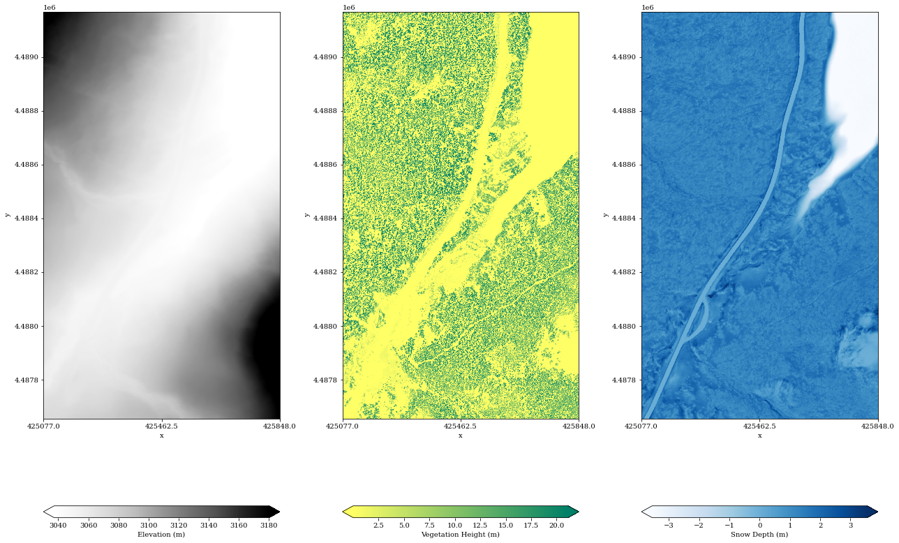
Let’s subset over small area for faster plotting and further analysis.
cam_dem_roi = cam_dem_snowFree.sel(y = slice(4489168, 4487655), x = slice(425077, 425848))
cam_vh_roi = cam_vh.sel(y = slice(4489168, 4487655), x = slice(425077, 425848))
cam_sd_roi = cam_snow_depth.sel(y = slice(4489168, 4487655), x = slice(425077, 425848))
# Set font size and font family
plt.rcParams.update({'font.size': 18})
plt.rcParams['font.family'] = 'serif'
plt.rcParams['font.serif'] = ['Times New Roman'] + plt.rcParams['font.serif']
#create fig and axes elements
fig, axs = plt.subplots(ncols = 3, figsize=(18, 12))
#plot the data
cam_dem_roi.plot(ax = axs[0], cmap = 'Greys', robust = True, cbar_kwargs={'label': 'Elevation (m)', 'orientation':'horizontal'})
cam_vh_roi.plot(ax = axs[1], cmap = 'summer_r', robust = True, cbar_kwargs={'label': 'Vegetation Height (m)', 'orientation':'horizontal'})
cam_sd_roi.plot(ax = axs[2], cmap = 'Blues', robust = True, cbar_kwargs={'label': 'Snow Depth (m)', 'orientation':'horizontal'})
#Set the title
# fig.suptitle('Cameron Study Area', fontsize = 20)
#set the axes title and tick locators
axs[0].set_title('')
axs[0].xaxis.set_major_locator(plt.LinearLocator(3))
axs[1].set_title('')
axs[1].xaxis.set_major_locator(plt.LinearLocator(3))
axs[2].set_title('')
axs[2].xaxis.set_major_locator(plt.LinearLocator(3))
plt.tight_layout()
plt.show()
More Analysis
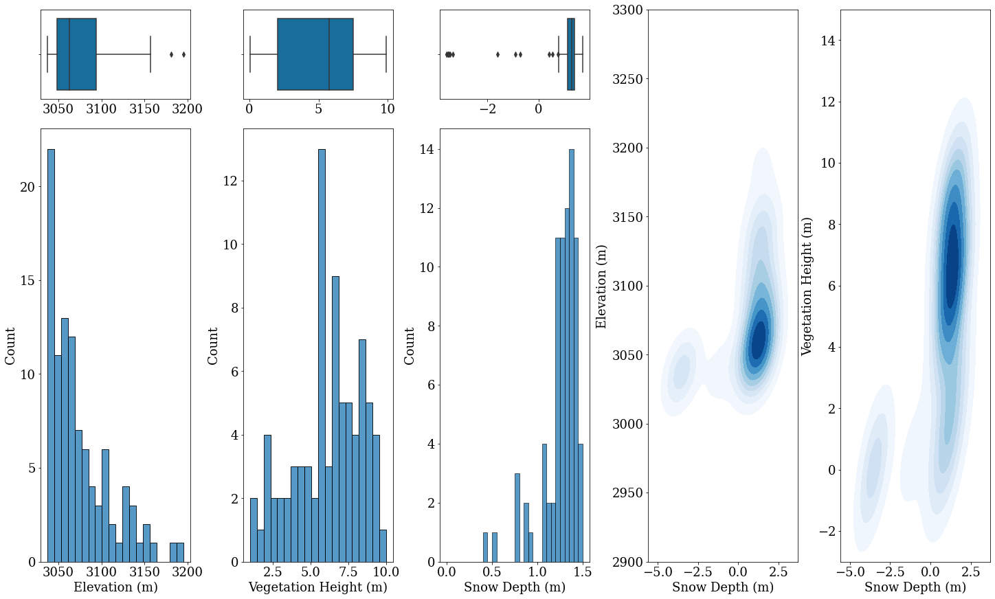
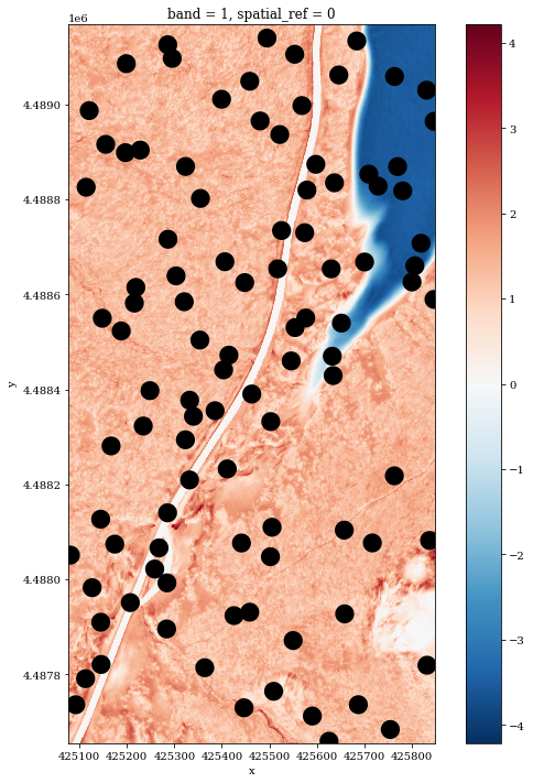
Lidar provides highly accurate DEM, vegetation height and snow depth. Our goal here is to quickly demonstrate some of the analysis we can do with these products. We will sample snow depth, elevation and vegetation height at 100 locations to quantify snow distribution over the the subset region
#import point location data
cam_100_points = gpd.read_file('/tmp/input/cameron_100_points.gpkg')
#create a dir to store the output
if not os.path.exists("./output"):
os.makedirs("./output")
#create a buffer around the point feature and save to file
cam_100_points.buffer(20).to_file('./output/cam_100_points_buffer.gpkg')
Let’s see the sampled points
cam_100_poly = gpd.read_file('./output/cam_100_points_buffer.gpkg')
fig, ax = plt.subplots(figsize=(10,12))
cam_sd_roi.plot(ax = ax)
cam_100_poly.plot(ax = ax, color = 'black')
plt.show()
#Extract raster values for the vegetation height
cam_VH_stat = rs.zonal_stats('./output/cam_100_points_buffer.gpkg',
cam_vh_roi.squeeze().values,
nodata = -9999,
geojson_out=True,
affine = cam_vh_roi.rio.transform(),
stats = 'count mean')
cam_VH_stat_df = gpd.GeoDataFrame.from_features(cam_VH_stat) #turn the geojson to a dataframe
cam_VH_stat_df.rename(columns = {'mean': 'VH_mean', 'count': 'VH_count'}, inplace = True) #rename the columns
#Extract raster values for the snow depth
cam_SD_stat = rs.zonal_stats(cam_VH_stat_df,
cam_sd_roi.squeeze().values,
nodata = -9999,
geojson_out=True,
affine = cam_sd_roi.rio.transform(),
stats = 'count mean')
cam_SD_stat_df = gpd.GeoDataFrame.from_features(cam_SD_stat) #turn the geojson to a dataframe
cam_SD_stat_df.rename(columns = {'mean': 'SD_mean', 'count': 'SD_count'}, inplace = True) #rename the columns
#Extract raster values for elevation
cam_DEM_stat = rs.zonal_stats(cam_SD_stat_df,
cam_dem_roi.squeeze().values,
nodata = -9999,
geojson_out=True,
affine = cam_dem_roi.rio.transform(),
stats = 'count mean')
cam_DEM_stat_df = gpd.GeoDataFrame.from_features(cam_DEM_stat) #turn the geojson to a dataframe
cam_DEM_stat_df.rename(columns = {'mean': 'ELEV_mean', 'count': 'ELEV_count'}, inplace = True) #rename the columns
#rename the dataframe
vh_sd_dem = cam_DEM_stat_df
# Set font size and font family
plt.rcParams.update({'font.size': 18})
plt.rcParams['font.family'] = 'serif'
plt.rcParams['font.serif'] = ['Times New Roman'] + plt.rcParams['font.serif']
#create figure and gridspec object
fig = plt.figure(figsize=(20,12), constrained_layout=True)
gspec = fig.add_gridspec(ncols=5, nrows=5)
ax0 = fig.add_subplot(gspec[0, 0])
ax1 = fig.add_subplot(gspec[0, 1])
ax2 = fig.add_subplot(gspec[0, 2])
ax3 = fig.add_subplot(gspec[1:5, 0])
ax4 = fig.add_subplot(gspec[1:5, 1])
ax5 = fig.add_subplot(gspec[1:5, 2])
ax6 = fig.add_subplot(gspec[0:5, 3])
ax7 = fig.add_subplot(gspec[0:5, 4])
# plot the boxplot of elevation, vegetation and snow thickness
sns.boxplot(x= vh_sd_dem['ELEV_mean'], ax=ax0, palette= 'colorblind')
ax0.set_xlabel('')
sns.boxplot(x= vh_sd_dem['VH_mean'], ax=ax1, palette= 'colorblind')
ax1.set_xlabel('')
sns.boxplot(x= vh_sd_dem['SD_mean'], ax=ax2, palette= 'colorblind')
ax2.set_xlabel('')
# plot the histogram and boxplot of elevation, vegetation and snow thickness
sns.histplot(data = vh_sd_dem, x ='ELEV_mean', ax=ax3, bins=20)
ax3.set_xlabel('Elevation (m)')
sns.histplot(data = vh_sd_dem, x ='VH_mean', ax=ax4, bins=20, binrange=(1,10))
ax4.set_xlabel('Vegetation Height (m)')
sns.histplot(data = vh_sd_dem, x ='SD_mean', ax=ax5, bins=30, binrange=(0,1.5))
ax5.set_xlabel('Snow Depth (m)')
#make the scatter plot of elevation vs snow thickness and vegetation vs snow thickness
sns.kdeplot(data = vh_sd_dem, x = 'SD_mean', y = 'ELEV_mean', shade=True, ax=ax6, cmap='Blues')
ax6.set_xlabel('Snow Depth (m)')
ax6.set_ylabel('Elevation (m)')
#set xlimit and y limit
#ax6.set_xlim(0, 2.5)
ax6.set_ylim(2900, 3300)
sns.kdeplot(data = vh_sd_dem, x = 'SD_mean', y = 'VH_mean', shade=True, ax=ax7, cmap='Blues')
ax7.set_xlabel('Snow Depth (m)')
ax7.set_ylabel('Vegetation Height (m)')
#set xlimit and y limit
#ax7.set_xlim(0, 2.5)
ax7.set_ylim(-3, 15)
plt.show()